Artificial Neural Networks for Interest Rate Forecasting based on Structural Change : A Comparative Analysis of Data Mining Classifiers

2003, Vol. 14, No.3 pp. 641∼651

Artificial Neural Networks for

Interest Rate Forecasting based on Structural Change:

A Comparative Analysis of Data Mining Classifiers ¹⁾

Kyong Joo Oh ²⁾

Abstract

This study suggests the hybrid models for interest rate forecasting using structural changes (or change points). The basic concept of this proposed model is to obtain significant intervals caused by change points, to identify them as the change-point groups, and to reflect them in interest rate forecasting. The model is composed of three phases. The first phase is to detect successive structural changes in the U. S.

Treasury bill rate dataset. The second phase is to forecast the change-point groups with data mining classifiers. The final phase is to forecast interest rates with backpropagation neural networks (BPN). Based on this structure, we propose three hybrid models in terms of data mining classifier: (1) multivariate discriminant analysis (MDA)-supported model, (2) case-based reasoning (CBR)-supported model, and (3) BPN-supported model. Subsequently, we compare these models with a neural network model alone and, in addition, determine which of three classifiers (MDA, CBR and BPN) can perform better. For interest rate forecasting, this study then examines the prediction ability of hybrid models to reflect the structural change.

Keywords: Backpropagation Neural Networks, Case-Based Reasoning, Multivariate Discriminant Analysis, Pettitt Test, Structural Change

1. Introduction

The prediction of interest rate is a vital task in managing financial activities.

To this end, traditional approaches have largely focused on statistical techniques

1) 본 연구는 2003학년도 한성대학교 사회과학연구원 특별연구비 지원과제임.

2) 서울시 성북구 삼선동3가 389번지 한성대학교 경영학부 전임강사

E-mail: [email protected]

such as exponential smoothing and moving averages. The need for better accuracy, however, has led to nonlinear techniques (Jaditz and Sayers, 1995), such as neural networks (Deboeck and Cader, 1994), fuzzy theory (Ju et al., 1997), and case-based reasoning (Kim and Noh, 1997). Previous work in the interest rate forecasting has tended to emphasize statistical techniques and artificial intelligent (AI) techniques in isolation over the past decades. However, an integrated approach, which makes full use of statistical approaches and AI techniques, offers the promise of improving performance over each method alone (Chatfield, 1993).

This study explores the ways in which such technologies may be combined synergistically, and illustrates the approach through the use of MDA, CBR and BPN as a data mining classifier. Up to now, it has been proposed that the hybrid model combining two or more models have a potential to achieve a high predictive performance in interest rate forecasting (Kim and Noh, 1997).

Interest rates is more fluctuated sensitively to government's monetary policy than other financial variable (Bagliano and Favero, 1999). Especially, banks play a very important role in determining the supply of money: Much regulation of these financial intermediaries is intended to improve its control. One crucial regulation is reserve requirements, which make it obligatory for all depository institutions to keep a certain fraction of their deposits in accounts with the Federal Reserve System, the central bank in the United States. It is supposed that government take an intentional action to control the currency flow which has direct influence upon interest rates. Therefore, we can conjecture that the movement of interest rates has a series of change points caused by the planned monetary policy of government.

On the basis of these characteristics of interest rate, this study suggests the change-point detection for interest rate forecasting. The basic concept of this proposed model is to obtain significant intervals occurred by change points, to identify them as the change-point groups, and to reflect them in interest rate forecasting. The proposed model consists of three phases: The first phase detects successive change points in interest rate dataset, the second phase forecasts the change-point groups with data mining classifiers, and the final phase forecasts the final output with BPN. According to the kind of data mining classifiers, we propose three hybrid models: (1) MDA-supported model, (2) CBR-supported model, and (3) BPN-supported model. Subsequently, we compare these models with a neural network alone, and determine which of three classifiers (MDA, CBR and BPN) can perform better. This study then examines the prediction ability of the hybrid models for interest rate forecasting using change-point detection, and compares the performance of several data mining classifiers.

We outline the development of change-point detection and its application to the

financial economics in Section 2. Section 3 describes the proposed hybrid model

details through the various data mining classifiers. Section 4 and 5 report the

procedures and the results of this study. Finally, the concluding remarks are

presented in Section 6.

2. Review of Structural Change in the Financial Economics

The detection and estimation of a structural or parametric change in forecasting is an important and difficult problem. In particular, financial analysts and econometricians have frequently used piecewise linear models which also include the change-point models. They are known as the models with structural breaks in the economics literature. In these models, the parameters are assumed to shift - typically once - during a fixed sample period and the goal is to estimate the two sets of parameters as well as the change point or structural break.

In order to detect the structural change, change-point detection methods have been applied to macroeconomic time series. Rapport and Reichlin (1989) and Perron (1989) conduct the first study in this field. From then on, several statistics have been developed which work well in a change-point framework, all of which are considered in the context of breaking the trend variables (Zivot and Andrew, 1992). In those cases where only a shift in the mean is present, the statistics proposed in Perron and Vogelsang (1992) stand out.

In spite of the significant advances by these works, we should bear in mind that some variables do not show just one change point. Rather, it is common for them to exhibit the presence of multiple change points. Thus, it seems advisable to introduce a large number of change points in the specifications of the models that allow us to obtain the abovementioned statistics. For example, Lumsdaine and Papell (1997) have considered the presence of two or more change points in trend variables. Based on this fact, we also assume the Treasury bill rates have two or more change points in our research model.

Up to now, there are few artificial intelligence models for financial applications to represent the change-point detection. Most of the previous research has a focus on the finding of unknown change points for the past, not the forecast for the future (Li and Yu, 1999). Our model finds change points in the training dataset and forecasts change points in the holdout dataset. It is demonstrated that the introduction of change points to our model will make the predictability of interest rates greatly improve.

3. Model Specification

3.1. The Basic Architecture of Proposed Model

Data mining classifiers, change-point detection method and neural network

learning method have been integrated to forecast the U. S. Treasury bill rates of

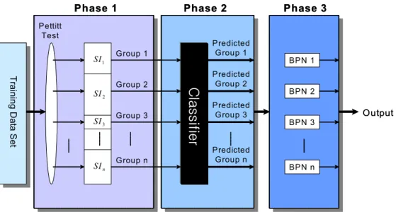
1 year's maturity. The advantages of combining multiple techniques to yield synergism for discovery and prediction have been widely recognized (Kaufman et al., 1991). The proposed models are determined by the kind of data mining classifier which is applied to the second phase of model. This section provides the architecture and the characteristics of our model (Figure 1) to involve the change-point detection and BPN.

In this study, a series of change-points will be detected by the Pettitt test (Pettitt, 1979), a nonparametric change-point detection method, since nonparametric statistical property is a suitable match for a neural network model that is a kind of nonparametric method. Based on the Pettitt test, the proposed model is composed of three phases as follows:

Figure 1. The Architecture of Proposed Model

Phase 1: Constructing homogeneous groups

It is known that interest rates at time t are more important than fundamental economic variables in determining interest rate at t + 1 (Larrain, 1991). Thus, we apply the Pettitt test to Treasury bill rates at time t in order to generate a forecast for t + 1 in the training dataset. The interval made by this process is defined as the significant interval, labeled SI, which is identified with a homogeneous group.

Step 1: Find a change point in 1∼N intervals by Pettitt test. If r

is a

Tr a ini ng Data S et

Phase 1 Phase 2

Pettitt Test

Group 1

SI

SI

SI

SI

BPN 1

BPN 2

BPN 3

BPN n

Phase 3

Output Predicted

Group 1

Group 2

Group 3

Group n

Predicted Group 2 Predicted

Group 3

Predicted Group n

C lassi fi er

Tr a ini ng Data S et

Phase 1 Phase 2

Pettitt Test

Group 1

SI

SI

SI

SI

BPN 1

BPN 2

BPN 3

BPN n

Phase 3

Output Predicted

Group 1

Group 2

Group 3

Group n

Predicted Group 2 Predicted

Group 3

Predicted Group n

C lassi fi er

change point, 1∼r

intervals are regarded as SI

and ( r

+ 1)∼N intervals are regarded as SI

. Otherwise, it is concluded that there does not exist a change point for 1∼N intervals. ( 1≤r

≤N)

Step 2: Find a change point in 1∼r

intervals by Pettitt test. If r

is a change point, 1∼r

intervals are regarded as SI

and (r

+ 1)∼r

intervals are regarded as SI

. Otherwise, 1∼r

intervals are regarded as

SI

like Step 1. ( 1≤r

≤r

)

Find a change point in ( r

+ 1)∼N intervals by Pettitt test. If r

is a change point, (r

+ 1)∼r

intervals are regarded as SI

and ( r

+ 1)∼N intervals are regarded as SI

. Otherwise, ( r

+ 1)∼N intervals are regarded as SI

like Step 1. ( r

≤r

≤N)

Step 3: By applying the same procedure of Step 1 and 2 to subsamples, we can obtain several significant intervals under the dichotomy if we need five or more significant intervals.

First of all, the number of structural change should be determined. If just one change point is assumed to occur in a given dataset, only the first step will be performed. Otherwise, all of the three steps will be performed successively. This process plays a role of clustering that constructs groups as well as maintains the time sequence. In this point, Phase 1 is distinguished from other clustering methods such as the k-means nearest neighbor method and the hierarchical clustering method. They classify data by the Euclidean distance between cases without considering the time sequence.

Phase 2: Group forecasting with data mining classifier

The significant intervals by Phase 1 are grouped to detect the regularities hidden in them and to represent the homogeneous characteristics of them. Such groups represent a set of meaningful trends encompassing the significant intervals.

Since those trends help to find regularities among the related output values more

clearly, the neural network model can have a better ability of generalization for

the unknown data. This is indeed a very useful point for sample design. In

general, the error for forecasting may be reduced by making the subsampling

units within groups homogeneous and the variation between groups heterogeneous

(Cochran, 1977). After Phase 1 detects the appropriate groups hidden in the

significant intervals, various classifiers (MDA, CBR and BPN) are applied to the

input data at time t with group outputs for t + 1. In this sense, Phase 2 is a

model that is trained to find an appropriate group for each given sample.

Phase 3: Forecasting the output with BPN

Phase 3 is built by applying the BPN model to each group. Phase 3 is a mapping function between the input at time t and the corresponding desired output (i.e. Treasury bill rates) at t + 1. Once Phase 3 is built, then the sample can be used to forecast the Treasury bill rates.

3.2. The Proposed Models by the Data Mining Classifiers

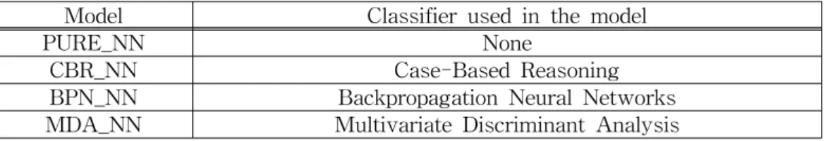
According to the kind of classifier used in the Phase 2, we propose three hybrid models: (1) MDA-supported model, (2) CBR-supported model and (3) BPN-supported model. The classifiers used in the proposed model are as shown in Table 1. In the second phase, these models applies CBR (Kolodner, 1991), BPN and MDA to forecast the change-point group using a commercial packages - Kate 5.02, NeuroShell 2 and SPSS 11, respectively.

Table 1. Models and their associated classifiers for the U.S. Treasury bill rate forecasting

Model Classifier used in the model

PURE_NN None

CBR_NN Case-Based Reasoning

BPN_NN Backpropagation Neural Networks

MDA_NN Multivariate Discriminant Analysis

4. Data and Variables

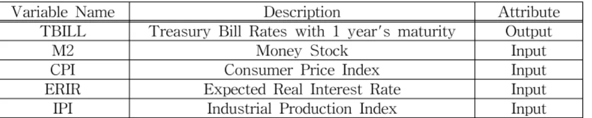
The input variables used in this study are money stock, consumer price index,

expected real interest rates and industrial production index. They are used in both

Phase 2 and Phase 3. The lists of variables used in this study are summarized in

Table 2. The data used in this study are obtained from the U. S. Federal Reserve

homepage (http://www.federalreserve.gov/releases/h15/data.htm). They are those

which were found significant in interest rate forecasting by previous study (Oh

and Han, 2001). To obtain stationary and thereby facilitate forecast, the input data

were transformed by a logarithm and a difference operation. Moreover, the

resulting variables were standardized to eliminate the effects of units.

Table 2. Description of Variables

Variable Name Description Attribute

TBILL Treasury Bill Rates with 1 year's maturity Output

M2 Money Stock Input

CPI Consumer Price Index Input

ERIR Expected Real Interest Rate Input

IPI Industrial Production Index Input

The training dataset includes observations from January 1961 to August 1991 while the holdout dataset runs from September 1991 to May 1999. The study employs two types of neural network models. The first type, labeled PURE_NN, involves input variables at time t to generate a forecast for t + 1. The input variables are M2, CPI, ERIR and IPI. The second type has the second-order learning model which consists of three phases mentioned in Section 3. The first learning is Phase 2 that forecasts the change-point group while the next learning is Phase 3 that forecasts the final output.

5. Empirical Results

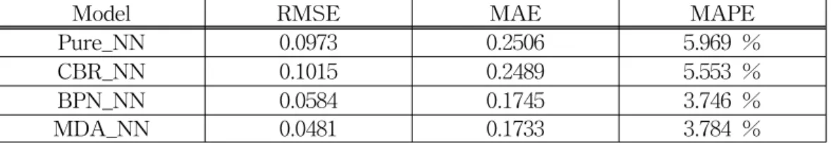
To highlight the performance due to the holdout data of various models, the

actual values of Treasury bill rates and their predicted values are shown in Figure

2 for the holdout dataset. The predicted values of PURE_NN and CBR_NN get

apart from the actual values in some intervals. Numerical values for the

performance metrics by predictive model are given in Table 3. According to root

mean squared error (RMSE), mean squared error (MAE) and mean absolute

squared error (MAPE), the outcomes indicate that BPN_NN and MDA_NN are

superior to PURE_NN and CBR_NN.

2 .5 3 3 .5 4 4 .5 5 5 .5 6 6 .5 7 7 .5

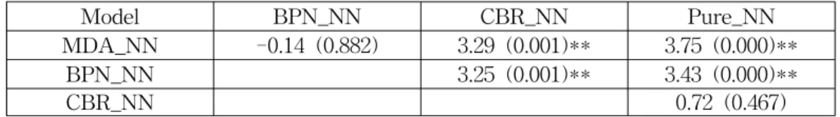
Sep-91 Dec-91 Mar-92 Jun-92 Sep-92 Dec-92 Mar-93 Jun-93 Sep-93 Dec-93 Mar-94 Jun-94 Sep-94 Dec-94 Mar-95 Jun-95 Sep-95 Dec-95 Mar-96 Jun-96 Sep-96 Dec-96 Mar-97 Jun-97 Sep-97 Dec-97 Mar-98 Jun-98 Sep-98 Dec-98 Mar-99

A c tu a l P u re _ N N C B R _ N N B P N _ N N M D A _ N N

Figure 2. Actual vs Predicted Values due to Various Models for TBILL

Table 3. Performance Results in the case of the U. S. Treasury bill rate forecasting based on RMSE, MAE and MAPE

Model RMSE MAE MAPE

Pure_NN 0.0973 0.2506 5.969 %

CBR_NN 0.1015 0.2489 5.553 %

BPN_NN 0.0584 0.1745 3.746 %

MDA_NN 0.0481 0.1733 3.784 %

Our approach to integration involves a multistrategy technique which may be called the second-order learning. Kim and Joo (1997) provided the good results with the second-order learning using CBR. However, CBR did not perform well in this study. In the second-order learning, the forecast from the superior method is selected on a case-by-case basis to determine the output of overall model. In other words, the second learning (BPN in this study) serves as a metalevel process to determine which of three elementary modules (CBR, BPN and MDA in this study) perform better. In this point, CBR is not a good elementary module.

Thus, we will choose BPN or MDA as the elementary modules for interest rate forecasting.

We use the pairwise t-test to examine whether there exist the differences in the predicted values of models according to the absolute percentage error (APE).

This metric is chosen since it is commonly used and is highly robust (Makridakis, 1993). Since the forecasts are not statistically independent and not always normally distributed, we compare the forecast's APEs using the pairwise t-test.

Where sample sizes are reasonably large, this test is robust to the distribution of

the data, to nonhomogeneity of variances, and to statistical dependence. Table 4 shows t-values and p-values when the prediction accuracies of the left-vertical methods are compared with those of the right-horizontal methods. It means that BPN_NN and MDA_NN perform significantly better than PURE_NN at a 1%

significant level. Furthermore, this suggests that the hybrid models using change-point detection can improve the performance by the use of the appropriate classifier.

Table 4. Pairwise t-tests for the differences in residuals for US interest rate prediction based on the absolute percentage error (APE)

with the significance level in parentheses.

Model BPN_NN CBR_NN Pure_NN

MDA_NN -0.14 (0.882) 3.29 (0.001)** 3.75 (0.000)**

BPN_NN 3.25 (0.001)** 3.43 (0.000)**

CBR_NN 0.72 (0.467)

** Significant at 1%

The neural network models using change-point detection turn out to have a high potential in interest rate forecasting. This is attributable to the fact that it categorizes the input data into homogeneous group and extracts regularities from each homogeneous group. Therefore, the neural network models using change-point detection can cope with the noise or irregularities more efficiently than PURE_NN. In addition, BPN and MDA perform very well as a classifier in interest rate forecasting.

6. Concluding Remarks

The proposed model has the promising possibilities to improve the performance if further studies are to focus on the various approaches in the construction and the prediction of the change-point groups. In the final phase of the model, other intelligent approaches can be used to forecast the final output besides BPN. In addition, the proposed models may be applied to other chaotic time series data, such as stock market prediction and exchange rate prediction. By the extension of these points, future research is expected to provide more improved neural network models with superior performances.

References

1. Bargliano, F. C., and Favero, C. A. (1999). Information from financial

markets and VAR measures of monetary policy, European Economic

Review, 43, 825-837.

2. Chatfield, C. (1993). Neural networks: Forecasting breakthrough or passing fad? International Journal of Forecasting, 9, 1-3.

3. Cochran, W. G. (1977). Sampling Techniques, Third edition, John Wiley

& Sons, New York.

4. Deboeck G., and Cader, M. (1994). Trading on the Edge, John Wiley &

Sons, New York.

5. Jaditz, T. and Sayers, C. L. (1995). Nonlinear in the interest rate risk premium, In R. R. Trippi, Chaos and Nonlinear Dynamics in the Financial Markets (pp. 335-357), Irwin.

6. Ju Y. J., Kim, C. E., and Shim, J. C. (1997). Genetic-based fuzzy models: interest rate forecasting problem, Computers and Industrial Engineering, 33(3-4), 561-564.

7. Kaufman, K. A., Michalski, R. S., and Kerschberg, L. (1991). Mining for knowledge in databases: Goals and general description of the INLEN system, In G. Piatetsky-Shapiro and W. J. Frawley (Eds), Knowledge Discovery in Databases (pp. 449-462), AAAI/MIT Press, Cambridge, MA.

8. Kolodner, J. (1991). Improving human decision making through case-based decision aiding, AI Magazine, 12, 52-68.

9. Kim S. H. and Noh, H. J. (1997). Predictabilityof interest rate using data mining tools: a comparative analysis of Korea and the US, Expert Systems with Application, 15, 85-95.

10. Kim, S. H. and Joo, J. (1997). Second-order learning for complex forecasting tasks: case study of Video-On-Demand, Korean Journal of Expert Systems, 3, 31-45.

11. Larrain, M. (1991). Empirical tests of chaotic behavior in a nonlinear interest rate model, Financial Analysts Journal, Sep.-Oct., 51-62.

12. Li, H. L. and Yu, J. R. (1999). A piecewise regression analysis with automatic change-point detection, Intelligent Data Analysis, 3, 75-85.

13. Lumsdaine, R. L. and Papell, D. H. (1997). Multiple trends and the unit root hypothesis, The Review of Economics and Statistics, 79, 212-218.

14. Makridakis, S. (1993). Accuracy measures: Theoretical and practical concerns, International Journal of Forecasting, 9, 527-529.

15. Oh, K. J., and Han, I. (2001). An Intelligent Clustering Forecasting System based on Change-Point Detection and Artificial Neural Networks:

Application to Financial Economics, Proceedings of the Thirty-Fourth Hawaii International Conference on System Sciences (HICSS), Hawaii, U.S.A.

16. Perron, P. (1989). The great crash, the oil price shock, and the unit root hypothesis, Econometrica, 57, 1361-1402.

17. Perron, P., and Vogelsang, T. (1992). Nonstationarity and level shifts

with an application to purchasing power parity, Journal of Business and Economic Statistics, 10, 301-320.

18. Pettitt, A. N. (1979). A non-parametric approach to the change-point problem, Applied Statistics, 28(2), 126-135.

19. Rapport, P., and Reichlin, L. (1989). Segmented trends and non-stationary time series, The Economic Journal, 99, 168-177.

20. Zivot, E., and Andrew, D. W. K. (1992). Further evidence on the great crash, the oil-price shocks, and the unit-root hypothesis, Journal of Business and Economic Statistics, 10, 251-270.

[ received date : Apr. 2003, accepted date : Jul. 2003 ]