Simple Material Budget Modeling for a River-Type Reservoir

Simple Material Budget Modeling for a River-Type Reservoir

Seong-Kyu Yoon⋅Dong-Soo Kong

^*,†

⋅Wookeun Bae

Department of Major in Civil and Environmental System Engineering, Hanyang University

*Department of Life Science, Kyonggi University

하천형 저수지의 단순 물질수지 모델링

윤성규ᆞ공동수

^*,†

ᆞ배우근

한양대학교 건설환경공학과

*경기대학교 생명과학과

(Received 3 November 2009, Revised 14 March 2010, Accepted 17 March 2010)

Abstract

Simple material budget models were developed to predict the dry season water quality for a river-type reservoir in Paldang, Republic of Korea. Of specific interest were the total phosphorus (TP), chlorophyll  (Chl. ), 5-day biochemical oxygen demand (BOD), and chemical oxygen demand (COD). The models fit quite well with field data collected for 20 years and have enabled the identification of the origins of organic materials in the reservoir. The critical hydraulic load that determines the usability of phosphorus for algal production appeared to be about 1.5 m d

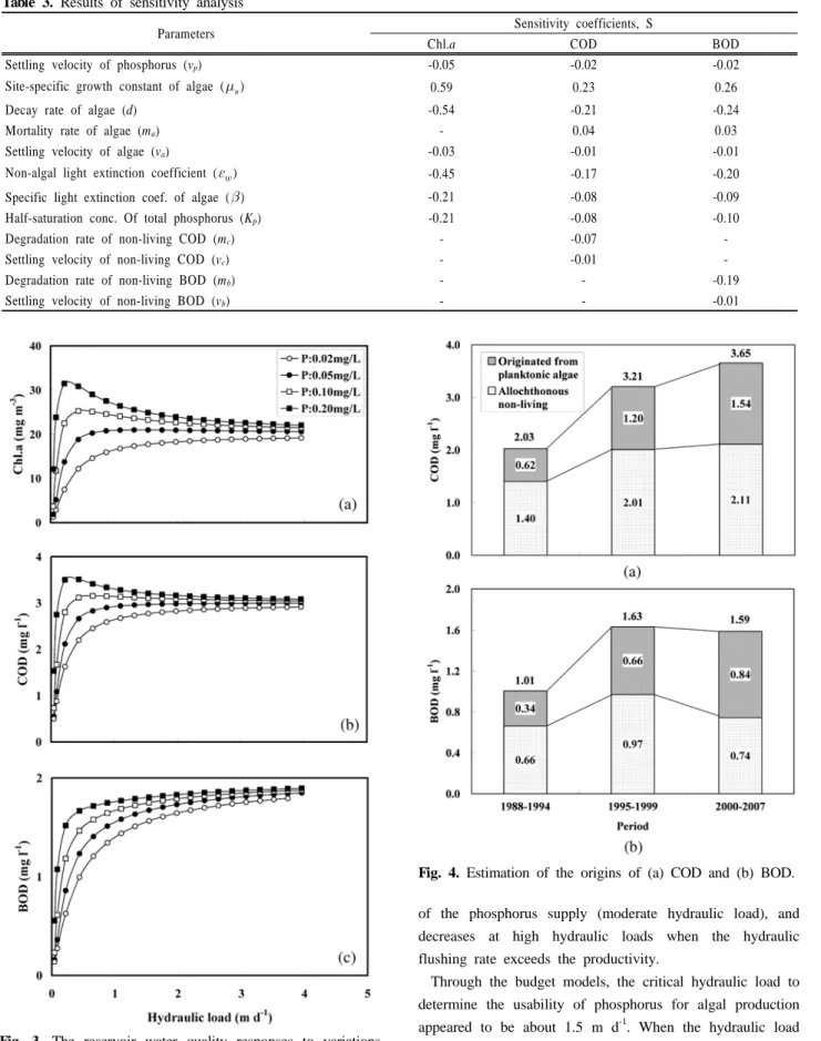
^-1

. When a hydraulic load was smaller than the critical value, the concentrations of Chl. , COD, and BOD in the reservoir water became sensitive to internal algal reactions such as growth, degradation, and settling. In spite of the recent intensive efforts for organic pollutant removal from major point sources by central and local governments, the water quality in the reservoir had not been improved. Instead, the concentration of COD increased. The model analysis indicated that this finding could be attributed to the continuing increase of the algal production in the reservoir and the allochthonous load from non-point sources. In particular, the concentrations of COD and BOD of algal origin during 2000~2007, each of which is comprised of approximately one half of the total, were approximately 2.5 times higher than those observed during 1988~1994 and approximately 1.3 times higher than those between 1995~1999.

The results of this study suggested that it is necessary to reduce the algal bloom so as to improve the water quality of the reservoir.

keywords : Eutrophication, Material budget modeling, Phosphorous, River-type reservoir, Water quality

1. Introduction

¹⁾

Previous studies on simple material budget models have focused mainly on the evaluation of the relationship bet- ween the concentration of phosphorus in lakes and its external loading (Dillon and Rigler, 1976; Kirchner and Dillon, 1975; Vollenweider, 1976). Vollenweider and Kerekes (1982) proposed empirical equations that relate the con- centration of phosphorus or algae in a lake to the average inflow concentration of phosphorus as a function of the average water residence time. Such models were developed for natural lakes, whose organic matter sources originate mainly from autochthonous algal production. In addition, most of these models are empirical in nature and have not been used outside the range of the data set employed for the model calibration (Kennedy and Walker, 1990).

†To whom correspondence should be addressed.

[email protected]

The water quality and productivity of an artificial reservoir are directly controlled to a large extent by the quantity and quality of external nutrient loadings (Thornton et al., 1990). In general, a reservoir is an open system connected, in many cases, to large rivers and watersheds. As such, organic sources of the reservoir are allochthonous as well as autochthonous. The algal and other organic material concentrations are often high due to pollutant loading and algal production during travel. Therefore, the construction of mass-balance equations in the reservoirs should, unlike natural lakes, consider the external loading of algae and organic materials. Previous non-linear regression equations for algal concentration in lakes were obtained as functions of expected total phosphorus concentration (Vollenweider and Kerekes, 1982) without considering the algal concen- tration from the inflow. Moreover, budget models for BOD and COD for a reservoir are rare.

The Paldang Reservoir is a shallow river-type reservoir

constructed in 1973 near the downstream of the Han River in the Republic of Korea. It is located about 45 km northeast of Seoul, and is the main water source for the domestic and industrial uses of the twenty four million people in the Seoul Metropolitan area. It has been partially eutrophicated since the 1980's, and its water quality has deteriorated particularly during periods of low flow in the spring.

The purpose of this study was to investigate the changes of the dry-season concentration of organic materials in the Paldang Reservoir while taking into account both external loadings and internal reactions. A material-budget model for algal concentration was developed as a function of inflow algal concentration, reservoir phosphorus concentra- tion, hydraulic coefficients, and related reaction parameters.

Material-budget models for BOD and COD were developed as functions of the predicted algal concentration in the reservoir and related parameters. The models were cali- brated and verified against field data that were collected during the spring season (March~May) for 20 years from 1988 to 2007.

2. Materials and methods

2.1. Description of the study area

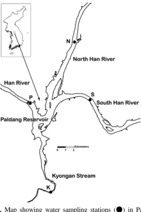
The Paldang Reservoir is located at the confluence of two rivers (North Han River and South Han River) and a stream (Kyongan Stream) at 127° 26E and 37° 29N (Fig. 1).

Fig. 1. Map showing water sampling stations (●) in Paldang Reservoir.

The entire watershed area of the reservoir reaches 23,600 km

²

. The mean depth of the reservoir is 6.5 m, and the surface area is 38.2 km

²

. The water level of the reservoir is maintained mostly between 25.0 ~ 25.5 m SEL. It has a high areal ratio (the area of the drainage basin to that of the reservoir surface) of 618. Thus, the water quality of the reservoir can be greatly influenced by the watershed pollutant loading. The reservoir has a high width-depth ratio of 104, providing a favorable condition for algal growth.

The annual mean flow rate entering the reservoir is 557 cubic meters per second (CMS), but is only 270 CMS when excluding the monsoon periods in June ~ September.

The hydraulic flushing rate and the hydraulic residence time (HRT) varied in the range of 41 ~ 140 (mean: 69) yr

^-1

and 2.6 ~ 9.0 (mean: 5.3) days, respectively. The flow rate to the reservoir in the spring was quite stable, as it was controlled by several upstream reservoirs (five reservoirs on the North Han River and two reservoirs on the South Han River) and the rainfall was light. The reservoir was polymictic and not stratified due to its short HRT and shallow depth, and was aerobic in all water columns (Kong, 1997).

The water quality of the three tributaries to the reservoir was quite different due to the unique pollution sources in the watersheds. Thus, three inflow sites (site N, S, K) and one outflow site (site P) were selected for sampling. Among them, site K and site P were located at the boundary of the reservoir and sites N and S were inside the reservoir.

Thus, the actual target area of this study for developing the budget models was reduced to the main body sur- rounded by the four sampling sites, of which the area was 19.7 km

²

with a mean water depth of 7.8 m.

2.2. Basic concept of material mass budget

In general, the material balance equation for a body of water that has multiple inflows and outflows can be expressed as

a o

o i

i

C Q C kVC L

dt Q VC

d ( ) = − − +

(1-1)

where

V : Water volume (L

³

)

C : Material concentration of a body of water (ML

^-3

) Q

i

: Inflow rate (L

³

T

^-1

)

 

_

: Flow-weighted average concentration of inflow material (ML

^-3

)

Q

o

: Outflow rate (L

³

T

^-1

)

 

_

: Flow-weighted average concentration of outflow

material (ML

^-3

)

k : Lumped first-order reaction coefficient (T

^-1

)

L

a

: Internal production of material in a body of water (MT

^-1

)

The main fraction of the Paldang Reservoir (surrounded by the four sampling sites) was simplified as a quasi- completely mixed system  ^{ }



≈   because it was polymictic and not stratified.

During spring, the rainfall is usually light in the watershed of the Paldang Reservoir and the inflow of the reservoir is constantly controlled by upstream reservoirs.

As a result, the flow and the materials load to the reser- voir were quite stable.

The water volume of the reservoir was, for the most part, maintained constant by the sluice gates and the nearby water-intake stations. The evaporation rate of the reservoir was very small when compared to the inflow rate because of the short HRT. Thus, the monthly inflow and outflow rates (including water intake) were almost equal (Q

i

≈ Q

o

≈ Q), and the body of water comprising the study area could be considered as a quasi-steady state system [(VC) / dt ≈ 0].

Based on the above simplifications and assumptions, Equation 1-1 becomes

(Input) Q C

_i

+ L

_a

= QC + kVC (Output) (1-2)

2.3. Equations for budget models 2.3.1. Total phosphorus

Total phosphorus can be assumed as a conservative material, but it can be removed by settling and biological consumption such as fishing in a body of water. Assuming that the biological consumption is relatively negligible, a budget model for total phosphorus can be constructed, as shown in Equation 2-1. An apparent settling rate, repre- sented as a lumped parameter in the equation, is analogous to a settling velocity divided by the mean water depth (k

p

= v

p

/ z).

p p p

pi

QC k VC

C

Q = + _(2-1)

where

 

_{ }

: Inflow total-phosphorus concentration (ML

^-3

) C

p

: Reservoir total-phosphorus concentration (ML

^-3

) k

p

: Lumped reaction coefficient for phosphorus (apparent

settling rate) (T

^-1

)

Rearranging for C

p

,

s p

pi s p

pi p

pi p

pi

p v q

C q z k

C Q Az k

C Q

V k C C

/ 1 / 1 ) / ( 1 ) / (

1 = +

= +

= +

= +

(2-2)

where

A : Surface area of the body of water (L

²

) Z : Mean water depth (L)

q

s

: Hydraulic load (Q / A (LT

^-1

)

v

p

: Apparent settling velocity of total-phosphorus (LT

^-1

)

2.3.2. Chlorophyll 

A mass balance equation for Chl.a can be expressed as follows.

a a a

ai

QC k VC

C

Q = + _(3-1)

s a

ai a

ai

a

k z q

C Q

V k C C

/ 1 ) / (

1 = +

= +

(3-2)

where

 

_

: Inflow Chl.a concentration (ML

^-3

) C

a

: Reservoir Chl.a concentration (ML

^-3

) k

a

: Lumped reaction coefficient for algae (T

^-1

)

The algal mass increases by photosynthesis, but decreases through respiration, death, predation, and settling. The lumped parameter k

a

encompasses those properties:

µ

− +

= d v z

k

_{a a}

/ _(3-3)

where

d : Decay (respiration, death, and predation) rate of algae (d

^-1

)

v

a

: Apparent settling velocity of algae (L T

^-1

)



: Specific growth rate of algae (d

^-1

)

The algal growth rate at a certain depth is determined by the light intensity, water temperature, and nutrient con- centration. In this study, the water temperature was not considered because its yearly variation for the Paldang Reservoir was insignificant in the spring seasons.

Since the light intensity diminishes with water depth in a turbid water body (shallow Secchi-disc depth in Table 1) such as the Reservoir Paldang, it was assumed that the algal growth was limited by the light intensity in water columns. Inhibition of algal growth by excessive light inten- sity was neglected.

Thus, dual monod-type limitation (Bae and Rittmann,

1996) by light and the limiting nutrient was adopted for

growth kinetics. Phosphorus was considered to be the sole

limiting nutrient because the Paldang Reservoir had a high nitrogen/phosphorus weight ratio of 18~44 (Kong, 1997).

This is much higher than the stoichiometric ratio (7.2) for algal synthesis (Redfield et al., 1963). Although algae take up inorganic phosphorus, organic phosphorus can be recy- cled for algal growth through mineralization in the re- servoir. Thus, the total phosphorus concentration calculated from Equation 2-2 was used in the following equation.

⎟ ⎟

⎠

⎞

⎜ ⎜

⎝

⎛

⎟⎟ +

⎠

⎜⎜ ⎞

⎝

⎛

= +

=

p p

p I

m p

m

K C

C I K C I

f I

f µ

µ

µ ( ) ( )

(3-4)

where

 : Specific growth rate of algae (T

^-1

)



_

: Maximum specific growth rate of algae (T

^-1

) f (I ) : Function of light intensity to algal growth f (C

p

) : Function of total-phosphorus concentration to

algal growth

K

I

: Half-saturation constant of light intensity (ly T

^-1

) (ly: langley = cal cm

^-2

)

K

p

: Half-saturation constant of total phosphorus (ML

^-3

)

In general, the light intensity in the water diminishes exponentially with water depth (Kalff, 2002).

z o

z

I e

I =

^−ε

_(3-5)

where

I

z

: Light intensity at water depth z (ly T

^-1

)

I

o

: Light intensity just below the water surface during daylight hours (ly T

^-1

)

 : Light extinction coefficient (L

^-1

)

The light extinction coefficient can be divided into two components, as shown in Equation 3-6 (Jørgensen, 1976).

a

w

β C

ε

ε = + _(3-6)

where



_

: Non-algal light extinction coefficient (L

^-1

)

 : Specific light extinction coefficient to Chl.a (L

²

M

^-1

)

Thus, the function of light intensity to algal growth at depth z becomes:

z C o I

z C o z o I

z o z I

z

a w

a w

e I K

e I e

I K

e I I K z I I

f

_{( )}

) (

) ,

(

_{ε β}

β ε ε

ε

+

− +

−

−

−

= +

= +

= +

(3-7)

Since the light intensity diminishes with water depth, the

growth rate of algae decreases with water depth. The varying light intensity can be averaged over the water column to calculate the mean growth rate of algae (Jørgensen, 1976).

⎟⎟⎠

⎜⎜ ⎞

⎝

⎛ +

+

= +

=

∫

_{− +}

z C o I

o I a

w z

a

e w

I K

I K z

C z

dz z I f z I

f ⁰ ln _{( )}

) (

) 1 , ( ) ,

( _{ε β}

β

ε

(3-8)

The light pattern at the surface can be expressed in terms of day length and average intensity or as a semi- sinusoidal curve, and the average intensity during daylight hours is likely to prove an acceptable approximation (James, 1984).

Applying the ratio of day length and considering the light intensity just below the water surface during daylight as a average value, the daily averaged light function can be expressed as follows.

⎟⎟ ⎠

⎜⎜ ⎞

⎝

⎛ +

+

= +

_{− + C z}

a I

a I a

w

a

e

w

I K

I K z

I C

f ln

_{( )}

) ) (

(

_{ε β}

λ β

ε φ

⎟

⎠

⎜ ⎞

⎝

⎛ +

+

= +

_{− + C z}

a w

a

e

w

z

C 1

^{( )}

ln 1 )

( λ

^{ε β}

λ β

ε φ

(3-9)

where

 : Fraction day that is daylight

I

a

: Average light intensity during daylight hours just below the water surface (ly T

^-1

)

λ : The ratio of light intensity (I

o

/ K

I

)

Substituting Equation 3-9 for Equation 3-4, the mean growth rate of algae becomes

p p

p z C a

w m

C K

C e

z

C

^{w a}

⎟ +

⎠

⎜ ⎞

⎝

⎛ +

+

= +

_{−( + )}

1 ln 1 )

( λ

^{ε β}

λ β

ε φ µ µ

(3-10)

From Equations 3-3 and 3-10, we find

[ ]

p p

p a

w

z C m

a

a K C

C C

v e dz z k

a w

+ +

+

− + +

= ^{− +}

β ε

λ λ φ

µ

ln(1 ) (1 ^{(ε β )} )

(3-11)

Substituting Equation 3-11 into Equation 3-2,

[ ]

p p

p a

w

z C m

a s a ai

s

K C

C C

v e dz C q

q C

a w

+ +

+

− + + +

=

^{− +}

β ε

λ λ φ

µ ln ( 1 ) ( 1

^{(ε β )}

)

(3-12)

In a turbid and deep body of water, the term e

^{−(εw+βCa)z}

in Equation 3-12 is close to 0. If e

^{−(εw+βCa)z}

is neglected

and µ

_m

φ ln( 1 + λ ) is considered to be a site-specific growth constant μ

_s

(since μ

_m

and K

I

are constants and seasonal mean I

o

and  do not vary much in a certain area), Equation 3-12 becomes

2

⎟ ⎟ − = 0

⎠

⎞

⎜ ⎜

⎝

⎛ −

− +

+

_{s ai a s w ai}

p p

p p w

a

q C C q C

C K

C µ C β ε

β ε δ

δ (3-13)

where δ = ^{β ( q}

^s

^{+ dz + v}

^a

⁾ .

Solving for the algal concentration,

2 /

2

4 ε δ

α

α

_{s w ai}

a

C C + + q

= (3-14)

where β

ε δ

β

α µ

^s

^C

^p

^K

^p

+ ^C

^p

+ ^q

^s

^C

^ai

−

^w

= /( )

.

Equation 3-14 is applicable to a turbid and moderately deep body of water. If a body of water is very shallow or transparent, the term e

^{−(εw+βCa)z}

cannot be neglected and Equation 3-12 should be used. In that case, there is no analytical solution for C

a

, but an approximate solution can be obtained using numerical methods or searching a target value in spreadsheet programs of computer.

2.3.3. Chemical oxygen demand

The non-living COD (excluding the COD from organic materials in living algae) concentration varies by advection, death and excretion of algae, degradation, settling, and release from sediment. In the Paldang Reservoir, the release of reduced inorganic substances such as methane and hydrogen sulfide to the water column from the sediment can be neglected since the reservoir is aerobic.

Thus, a mass balance equation for non-living COD in the reservoir can be expressed as

cn c c cn a a c

cni

R m VC QC m v z VC

C

Q + = + ( + / ) _(4-1)

where

 

_{ }

: Inflow non-living COD concentration (ML

^-3

) R

c

: COD conversion factor of algae

m

a

: Mortality rate of algae (T

^-1

)

C

cn

: Reservoir non-living COD concentration (ML

^-3

) m

c

: Degradation rate of non-living COD (T

^-1

) v

c

: Settling velocity of non-living COD (LT

^-1

)

The COD conversion factor of algae (R

c

) depends on the

content ratio of carbon to Chl.a of algae (R

ca

), the stoichiometric ratio of oxygen to carbon of algae (R

oc

), and the KMnO

4

-oxidation ratio of algal carbon (R

oxi

).

oxi oc ca

c

R R R

R = _(4-2)

It was impossible to measure the non-living COD con- centration from the sample water that contained algae, because living algae in the water sample cannot be physically separated from the particulate non-living organic matters. Thus, non-living COD concentration should be calculated from other measured data. In this study, the concentration of non-living COD in the inflow water was calculated with the concentration of COD, the concen- tration of Chl.a, and the COD conversion factor.

ai c ci

cni

C R C

C = − _(4-3)

where

 

_

: Inflow COD concentration (ML

^-3

)

Then, from Equations 4-1 and 4-3, the reservoir non- living COD concentration is determined as follows.

c c s

a a c ai c ci s

cn

q m z v

zC m R C R C C q

+ +

+

= ( − )

(4-4)

The COD concentration in the reservoir water can be calculated by adding the algal COD to the non-living COD. Thus, the final budget model for the COD becomes

( )

a c c

c s

a a c ai c ci s

c

R C

v z m q

zC m R C R C

C q +

+ +

+

= −

(4-5)

where

C

c

: Reservoir COD concentration (ML

^-3

)

Assuming C

a

= 0 in Equation 4-5, organic materials from dead and living algae in the reservoir were excluded. As organic materials of the inflow algae were deducted in the same equation, an assumption of C

a

= 0 leads to calculated values that become the reservoir non-living COD or BOD concentration originating from an allochthonous load

( )

c c s

ai c ci s

cna

q m z v

C R C C q

+ +

= −

(4-6)

where

C

cna

: Reservoir non-living COD concentration originating from an allochthonous load (ML

^-3

)

2.3.4. Biochemical oxygen demand

A budget model for BOD will be similar to that for COD except for the conversion factors.

bn b

b bn a a bm

bni

R m VC QC m v z VC

C

Q + = + ( + / ) _(5-1)

where

C

bni

: Inflow non-living BOD concentration (ML

^-3

) R

bm

: BOD conversion factor of dead algae

C

bn

: Reservoir non-living BOD concentration (ML

^-3

) m

b

: Degradation rate of non-living BOD (T

^-1

) vb : Settling velocity of non-living BOD (LT

^-1

)

The BOD conversion factor of dead algae (R

bm

) depends on R

ca

, R

oc

, and the bacterial decomposition of dead algae during incubation for 5 days.

) 1 (

^5mbb

oc ca

bm

R R e

R = −

⁻

_(5-2)

where

m

bb

: Decomposition rate of dead algae at 20°C bottle (T

^-1

)

The non-living BOD concentration was calculated through the use of Equation 5-3.

ai br bi

bni

C R C

C = − _(5-3)

where

C

bi

: Inflow BOD concentration (ML

^-3

) R

br

: BOD conversion factor of living algae

The BOD conversion factor of living algae (R

br

) depends on R

ca

, R

oc

, and the endogenous respiration ratio of living algae during incubation for 5 days.

) 1 (

^5r

oc ca

br

R R e

R = −

⁻

_(5-4)

where

r : Endogenous respiration rate of living algae at 20°C bottle (T

^-1

)

From Equations 5-1 and 5-3, the reservoir non-living BOD concentration can be written as follows.

b b s

a a bm ai br bi s

bn

q m z v

zC m R C R C C q

+ +

+

= ( − )

(5-5)

By adding algal BOD to non-living BOD in the water, we obtain

( )

a br b

b s

a a bm ai br bi s

b

R C

v z m q

zC m R C R C

C q +

+ +

+

= −

(5-6)

where

C

b

: Reservoir BOD concentration (ML

^-3

)

Assuming Ca = 0 in Equation 5-6, the reservoir non- living BOD concentration originating from an allochthonous load is obtained as follows.

( )

b b s

ai br bi s

bna

q m z v

C R C C q

+ +

= −

(5-7)

where

C

bna

: Reservoir non-living BOD concentration originating from an allochthonous load (ML

^-3

)

2.4. Sampling and measurements

Water samples were collected weekly, biweekly, or monthly from several water depths at each site during March~May from 1988 to 2007.

The Secchi-disc depth (Z

SD

) was measured on-site with a white Secchi-disc (30 cm in diameter). The following four water quality variables were measured in the laboratory:

the concentrations of TP (ascorbic acid method after persulfate digestion), Chl.a (Spectrophotometric determina- tion of chlorophyll), BOD (5-day BOD test), and COD (oxidized by KMnO

4

). The first three variables were determined following the Standard Methods (APHA, 2005).

The COD concentration was determined by the potassium permanganate method (Klein, 1973). Above-all measure- ment was conducted by Han River Environment Research Center (unpublished).

2.5. Statistical analysis

The confidence level of a model is often evaluated by regression of the simulated results against the observed data. However, the regression coefficient can be high, although the simulated values are not similar to the observed values. Thus, the coefficient of E proposed by Nash and Sutcliffe (1970) was used in this study. Unless each value of the simulation fits the corresponding observation well, the Nash-Sutcliffe coefficient becomes low even in cases where the regression coefficient is high.

The range of E values lies between 1.0 (perfect fit) and

 ∞(absolute unfit). If the E value is below zero, the

Table 1. Annual variations of hydraulic load (q

s

) and water quality parameters (mean values of data measured weekly or biweekly during spring at site P).

Year qs

(m d^-1)

TP (mg m^-3)

Chl.a (mg m^-3)

ZSD

(m)

_ (m^-1)



(m^-1)

COD (mg l^-1)

BOD (mg l^-1)

1988 0.66 18 5.1 3.24 0.10 0.42 2.73 1.13

1989 1.13 24 7.6 1.98 0.15 0.71 2.12 1.09

1990 2.73 31 7.3 1.56 0.15 0.95 1.73 1.00

1991 1.62 56 7.7 1.65 0.15 0.88 1.43 0.87

1992 1.78 52 12.0 1.39 0.24 0.99 1.57 1.00

1993 1.93 39 15.3 1.32 0.31 0.99 2.05 1.27

1994 1.09 31 11.3 1.27 0.23 1.12 2.28 1.23

1995 1.25 31 21.2 1.37 0.42 0.82 2.62 1.30

1996 1.12 21 12.1 1.52 0.24 0.88 3.00 1.33

1997 1.53 44 15.1 1.18 0.30 1.13 3.38 1.83

1998 2.18 43 29.3 1.20 0.59 0.83 3.47 1.85

1999 1.66 37 25.2 1.77 0.50 0.46 3.12 1.78

2000 1.00 32 15.8 1.66 0.32 0.71 3.36 1.64

2001 0.90 51 23.9 1.31 0.48 0.82 3.55 1.44

2002 1.10 51 24.4 1.19 0.49 0.93 3.52 1.47

2003 2.40 40 23.8 1.17 0.48 0.98 2.86 1.32

2004 1.26 44 31.6 1.27 0.63 0.71 4.33 1.71

2005 0.95 36 27.4 1.46 0.55 0.62 4.46 1.47

2006 1.23 50 27.5 1.34 0.55 0.72 3.92 1.79

2007 1.36 52 22.3 1.14 0.45 1.04 3.69 1.67

ZSD : Secchi-disc depth, _ : light extinction coefficient due to algae,  : non-algal light extinction coefficient

accuracy of the model is considered low.

∑ ∑

∑ ∑

∑ −

− −

− =

−

−

= −

² ₂ ² ₂²

) (

) 1 (

) (

) ( ) (

C C

C C C

C

C C C

E C

^{s s}

(6-1)

where

E : Nash- Sutcliffe coefficient C : Mean of observed values C : Observed value

C

s

: Simulated value

The sensitivity of the model was examined using Equation 6-2 (Orlob, 1983). The relationship was norma- lized by introducing a nominal reference value ω for each parameter. This would give a nominal reference value C

ω

for the predicted state variable response. In this study, the sensitivity of the suggested models was tested for 50%

and 150% of the reference values of parameters.

ω ω ω ω ω ω ω

ω

ω ω ω ω

ω C

C C C C C C

S C

^{1.5 0.5 1.5 0.5}

/

) 5 . 0 5 . 1 (

/ ) (

/

/ = −

−

= −

∆

= ∆

(6-2)

where

S : Sensitivity coefficients

ω : Reference values of parameters

C

ω

: Predicted values for reference parameter value ω

3. Results and Discussion

3.1. Water quality

The correlation was weak among the standing crop of algae, transparency, and total phosphorus concentration during low flow periods (Table 1). The value of the non- algal light extinction coefficient by water and soluble and particulate matters (

_

) was three times higher than that displayed by algae ( 

_

). The 

_

and phosphorus concen- tration tended to vary with the hydraulic load such that phosphorus could be a limiting factor for algal growth at a condition of low hydraulic load. On the other hand, light intensity could be a limiting factor at a high hydra- ulic load. These results confirmed that hydrological factors such as turbidity and discharge are the primary factors to control water quality in a river-type reservoir (Winston and Criss, 2002).

3.2. Estimations of model parameters

The apparent settling velocity of total phosphorus (v

p

)

can be calculated from Equation 2-2. In the Paldang Reser-

voir, the mean apparent settling velocity of phosphorus

during March~May from 1988 to 2007 was 0.38 m d

^-1

,

and the apparent settling rate (the settling velocity divided

by the mean depth (7.8 m)), was 0.049 d

^-1

. The retention

coefficient of phosphorus, R (= 1 - C

p

/ C

pi

) appeared to be

Table 2. Parameter values calibrated in material budget models in the study reservoir

Parameters Units Calibrated values

TP

(Cp) Settling velocity of total phosphorus (vp) md^-1 0.38

Algae (Ca)

Maximum specific growth rate (



_) d^-1 2.0

Fraction day that is daylight (



) - 0.55

Ratio of light intensity (

λ

) - 3.7

Site-specific growth constant (



_) d^-1 1.7

Decay rate (d) d^-1 0.08

Mortality rate (ma) d^-1 0.02

Settling velocity (va) md^-1 0.05

Non-algal light extinction coefficient (



_) md^-1 0.84 Specific light extinction coef. of algae (



) m² (mg Chl.a)^-1 0.02 Half-saturation conc. of total phosphorus (Kp) mg L^-1 0.02 COD

(Cc)

Degradation rate of non-living COD (mc) d^-1 0.02 Settling velocity of non-living COD (vc) md^-1 0.02 COD conversion factor of algae (Rc) mg l^-1COD / mg m^-3 Chl.a 0.056 BOD

(Cb)

Degradation rate of non-living BOD (mb) d^-1 0.08 Settling velocity of non-lining BOD (vb) md^-1 0.02 BOD conversion factor of algae (Rbm, Rbr) mg l^-1 BOD / mg m^-3 Chl.a 0.031

0.22 ± 0.09 (mean ± standard deviation).

The apparent settling velocity of total phosphorus in the reservoir was approximately 10 times higher than that reported in natural lakes (Vollenweider, 1975: 10 m yr

^-1

, Dillon and Kirchner, 1975: 13.2 m yr

^-1

, Chapra, 1975: 16 m yr

^-1

). This was likely due to the inflow, which, in comparison to natural lakes, contained a relatively large amount of soil particles that acted as phosphorus carriers.

Although the apparent settling velocity of phosphorus was high, the phosphorus retention coefficient in the reservoir was relatively low compared to 0.2~0.5 in the natural lakes (Larsen et al., 1981) or 0.59 in the deep-reservoir Soyang in Korea (Heo et al., 1992). It seems that soil particles in the reservoir were very advective due to a short HRT and a fast flow velocity.

Kong (1992) reported that the mean value of the daily incident light intensity on the water surface was 395 ly d

^-1

and the mean value of the daylight fraction () was 0.55 in the Paldang Reservoir during March~May. Thus, the average incident light intensity during daylight hours on the water surface was approximately 718 ly d

^-1

(=395/0.55 ly d

^-1

). When the value of albedo on the water surface is 0.1 (Talling, 1957), the average incident light intensity during daylight hours just below the water surface (I

a

) was estimated as approximately 646 ly d

^-1

(=0.9×718 ly d

^-1

).

The saturating light intensity for algal photosynthesis was recommended as the range of 200 ~ 500 ly d

^-1

in the WASP5 model (Ambrose et al., 1993). The value of 175 ly d

^-1

for the half-saturation constant of light (K

I

) was used in this study, and it is identical to a half of the

mean value in the above-mentioned range of saturating light intensity. Thus, the value of 3.7 (=646/175) for the ratio of light intensity ( λ ) was used.

The vertical light extinction coefficient is usually esti- mated from the Secchi-disc depth as ε = 1.7 / Z

SD

(Wetzel, 1983). Megard et al. (1980) reported that the specific light extinction coefficient to Chl.a () in Equation 3-6 was in the range of 0.009~0.02 m

²

mg

^-1

. In this study, the  value, estimated from a regression of the observed light extinction coefficient estimated from the Secchi-disc depth versus Chl.a using Equation 3-6, was 0.02 m

²

mg

^-1

. It is the same as that reported by Lorenzen (1980) and similar to the 0.017 m

²

mg

^-1

recommended in the WASP5 model (Ambrose et al., 1993). This value is also similar to the 0.018 m

²

mg

^-1

reported for the Paldang Reservoir by Kong (1992).

In this study, the value of 30 for the content ratio of carbon to Chl.a of algae (R

ca

) and 2.67 for the stoichio- metric ratio of oxygen to carbon of algae (R

oc

) was used (Ambrose et al., 1993). Kim et al. (2007) reported that the KMnO

4

-oxidation ratio of algal carbon (R

oxi

) was 0.7±0.3 (mean±standard deviation) during the spring seasons in the two upper reservoirs of the Paldang Reservoir. From the result, the value of 0.7 for R

oxi

was used in this study.

Thus, the COD conversion factor of algae (R

c

) becomes about 0.056 mg l

^-1

COD to 1 mg m

^-3

Chl.a.

In this study, a value of 0.1 d

^-1

was used for the de-

composition rate (m

bb

) and the endogenous respiration rate

(r), resulting in a BOD conversion factor of dead algae

(R

bm

) and BOD conversion factor of living algae (R

br

) of

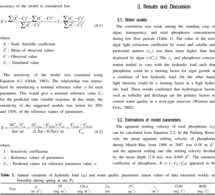
Fig. 2. Calibration and verification results of simple budget models (calibrated with data during 1988~1997, verified against data during 1998~2007).

approximately 0.031 mg l

^-1

BOD to 1 mg m

^-3

Chl.a.

3.3. Calibration and verification

The reaction coefficients in each budget model were calibrated by trial and error with the mean data obtained during the spring seasons from 1988 to 1997. These coefficients were verified with data during the spring seasons from 1998 to 2007. The calibrated values of all reaction coefficients are given in Table 2.

Because the study area was highly turbid and its mean water depth was moderate (about 8 m), there was little discrepancy between the solutions given by Equation 3-14 and a numerical method of Equation 3-12 for C

a

(the mean data error of solutions given by Equation 3-14 for numerical solutions: 0.03%). Thus, all solutions were obtained from Equation 3-14.

The calculated values for most of the materials by the budget models fit the observed values quite well (Fig. 2).

The model efficiency in calibration, evaluated with the Nash-Sutcliffe coefficient (E), was high and in the range of 0.83-0.88 for all parameters. It deteriorated to some degree in verification except for COD. Overall, the model predictions were quite close to the data and ideally re- presented the fluctuations of the contaminant concentration over the years.

Table 3 shows the results of sensitivity analysis on Chl.a, COD, and BOD. The maximum specific growth and decay rate of algae, as well as the non-algal light extinc- tion coefficient were the moderately sensitive parameters.

The settling velocities for phosphorus, algae, and non- living COD and BOD were insensitive. In general, the Chl.a concentration was more sensitive to the parameters than were the COD and BOD concentrations.

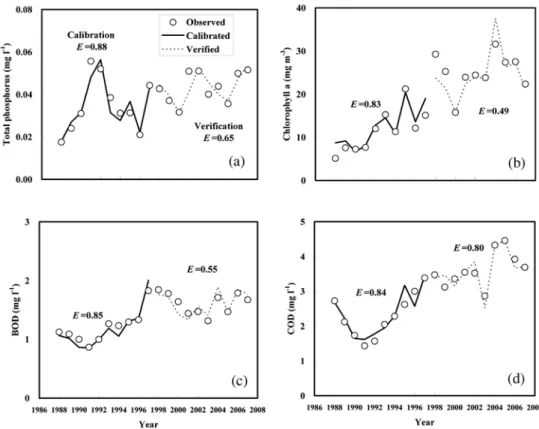
3.4. Scenario analysis

The changes of the reservoir Chl.a, COD, and BOD concentrations following changes in hydraulic load and inflow phosphorus concentration were simulated (Fig. 3).

At a hydraulic load over 1.5 m d

^-1

, the concentrations of Chl.a, COD, and BOD reach a level of inflow concentr- ation irrespective of the inflow total phosphorus concentration.

With a low concentration of inflow phosphorus (0.02 mg

l

^-1

), the contaminant concentrations decrease with a de-

crease of the hydraulic load. At a moderate (0.1 mg l

^-1

) or

high (0.2 mg l

^-1

) concentration of inflow phosphorus, Chl.a

and COD increase as the hydraulic load decreases before

they fall abruptly as the hydraulic load further decreases to

zero. This result indicates that algal concentration decreases

due to low productivity at a low supply of phosphorus (low

hydraulic load), reaches a peak value with an increase

Table 3. Results of sensitivity analysis

Parameters Sensitivity coefficients, S

Chl.a COD BOD

Settling velocity of phosphorus (vp) -0.05 -0.02 -0.02

Site-specific growth constant of algae (



_) 0.59 0.23 0.26

Decay rate of algae (d) -0.54 -0.21 -0.24

Mortality rate of algae (ma) - 0.04 0.03

Settling velocity of algae (va) -0.03 -0.01 -0.01

Non-algal light extinction coefficient (



_) -0.45 -0.17 -0.20 Specific light extinction coef. of algae (



) -0.21 -0.08 -0.09 Half-saturation conc. Of total phosphorus (Kp) -0.21 -0.08 -0.10

Degradation rate of non-living COD (mc) - -0.07 -

Settling velocity of non-living COD (vc) - -0.01 -

Degradation rate of non-living BOD (mb) - - -0.19

Settling velocity of non-living BOD (vb) - - -0.01

Fig. 3. The reservoir water quality responses to variations in hydraulic loads and the inflow total phosphorus concentrations (0.02, 0.05, 0.1, 0.2 mg l

^-1

) at the condition of (a) Chl.a; 20 mg m

^-3

, (b) COD; 3 mg l

^-1

, (c) BOD; 2 mg l

^-1

in the inflow.

Fig. 4. Estimation of the origins of (a) COD and (b) BOD.

of the phosphorus supply (moderate hydraulic load), and decreases at high hydraulic loads when the hydraulic flushing rate exceeds the productivity.

Through the budget models, the critical hydraulic load to

determine the usability of phosphorus for algal production

appeared to be about 1.5 m d

^-1

. When the hydraulic load

is above the critical value, the reservoir Chl.a, COD, and

BOD concentrations were not sensitive to the inflow total

phosphorus concentrations or internal reactions such as

production, degradation, and settling.

The origins of COD and BOD in the reservoir can be divided stepwise from budget models. The reservoir non- living COD or BOD concentration originating from an allochthonous load can be obtained by Equation 4-6 or Equation 5-7. The COD or BOD concentration originating from algae can be estimated by subtracting the he above- mentioned allochthonous non-living COD or BOD concen- tration from the COD or BOD concentration expected in Equation 4-5 or Equation 5-6.

In the reservoir, the non-living BOD concentration origi- nating from the allochthonous load increased during 1995~

1999, but tended to decrease after 2000 (Fig. 4). This may be attributed to pollution control measures, such as the activated sludge treatment of domestic sewage through intensive governmental plans after 1999. However, non- living COD concentration originating from the allochthonous load increased slightly after the plans. This may have occurred because the increase of COD load from non-point sources was higher than the decrease of COD load from the point sources.

Algae-originated COD and BOD concentrations have increased continuously in the reservoir. Algae-originated COD and BOD concentrations during 2000~2007 appeared to be 1.54 mg l

^-1

(42% of total COD) and 0.84 mg l

^-1

(53% of total BOD), respectively. They were 2.5 times higher than that during 1988~1994 and 1.3 times higher than that during 1995~1999.

In spite of the intensive domestic sewage control efforts by central and local governments since 1999, the COD concentration in the reservoir increased by more than 10%.

The BOD concentration decreased slightly, but did not meet to the target level (1.0 mg l

^-1

). This may be a result of the high algal production through eutrophication and the allochthonous load from non-point sources mentioned above.

4. Conclusion

In the shallow river-type reservoir Paldang, the simple material budget models for total phosphorus, chlorophylla, 5-day biochemical oxygen demand, and chemical oxygen demand demonstrated good predictability for field obser- vations, and enabled identification of the origins of organic materials in the reservoir.

Algal concentration in the reservoir appeared to depend on the supply of phosphorus and the flushing rate. When the hydraulic load was over the critical point (1.5 m d

^-1

), the reservoir Chl.a, COD, and BOD concentrations were not sensitive to the inflow total-phosphorus concentration due to the high flushing rate. When it was below the critical point, the reservoir Chl.a, COD, and BOD

concentrations were sensitive to the inflow total-phosphorus concentrations.

In spite of the intensive domestic sewage control efforts (mainly BOD reduction by activated sludge treatment) by central and local governments since 1999, the COD concentration in the reservoir has increased. The BOD concentration has decreased slightly, but still failed to meet the target level. This may have been largely due to the increase of eutrophication and allochthonous load from non-point sources. From the budget models, the concentra- tions of algal-origin COD and BOD during 2000~2007 were higher than that during previous periods. This indi- cated that control of algal bloom is critical for an improvement in the water quality of the Paldang Reservoir.

Although the calculated values by the budget models fit the observed values quite well, the proposed models have several limitations; one box model assuming a quasi-com- pletely mixed system, simplified algal growth kinetics (neglect of phosphorus speciation), simplified solar radia- tion conditions, neglect of sediment interaction, etc. If any water body is very shallow or transparent, a correction factor should be added to the model. Thus, the models will be available to polymictic water body with moderate depth such as Reservoir Paldang.

국문요약

하천형 저수지인 팔당호의 건기시 수질을 모의하기 위하 여 단순 물질수지 모델을 개발하였다. 대상 물질은 총인 (TP), 클로로필a (Chl.a), 5일 생물학적 산소 요구량 (BOD) 화학적 산소요구량 (COD)이었다. 모델은 지난 20년간의 실 측치를 잘 재현하였으며 유기물질의 성인을 밝히는데 이용 될 수 있었다. 모델을 통하여 분석한 결과, 팔당호에서 인 에 대한 조류의 이용성을 결정하는 임계 수리부하는 약 1.5 m d

^-1

로 나타났다. 팔당호의 Chl.a, COD, BOD 농도는 임계부하보다 작은 수리부하의 조건에서 생산과 호흡 및 침전과 같은 조류의 변화에 민감하게 반응하였다. 최근 유 기오염 저감을 위한 중앙정부와 지방정부의 강도 높은 노 력에도 불구하고 팔당호의 수질은 크게 개선되지 않았으며 오히려 COD 농도는 증가하였다. 모델 해석을 통하여 이는 조류 생산량의 증가와 아울러 비점오염원 등에서 외래성 부하가 증가하였기 때문인 것으로 나타났다. 특히 2000~

2007년 기간의 조류 기원성 유기물 농도는 전체 유기물 농 도의 절반에 해당하는 것으로 추정되었으며, 이는 1988~

1994년 기간에 비하여 2.5배, 1995~1999년 기간에 비하여

1.3배에 달하는 수준이었다. 이러한 연구의 결과는 팔당호

의 수질개선을 위해서는 조류 발생을 억제하는 것이 필요

함을 시사하는 것이었다.