Assessing the Utility of Rainfall Forecasts for
Weekly Groundwater Level Forecast in Tampa Bay Region, Florida 주단위 지하수위 예측 모의를 위한 강우 예측 자료의 적용성 평가:
플로리다 템파 지역 사례를 중심으로
Hwang, Syewoon*,**,†․Asefa, Tirusew***․Chang, Seungwoo* 황세운․아세파 터루소․장승우
ABSTRACT
미래 기후 정보를 이용한 수문 환경의 단기 미래 예측은 안정적 수자원 공급을 위한 필수적 과제이다. 미국 플로리다 주 중서부 템파 지역에서는 주요 수자원 중 하나인 지하수의 효과적 활용을 위해 지하수위 인공신경망 모델 (GWANN)을 개발하여 피압 대수층과 비 피압 대수층에 대한 주 단위 평균 지하수위를 월별로 예측하고 그 결과를 수자원 공급 의사 결정에 반영하고 있다. 본 논문은 템파지 역에 대한 GWANN 모델을 이용한 지하수위 예측 시스템을 소개하고 모델의 기후 입력 자료의 민감도를 분석함으로써 양질의 기후 정 보에 대한 현 시스템의 활용성을 검토하였다. 2006년과 2007년에 대한 연구 결과, 관측 자료를 최적 예측 시나리오 (the best forecast) 로 가정하여 적용한 결과는 지하수위 관측 지점에 따라 큰 차이를 보였지만 일반적으로 현 시스템 (현 시점의 실시간 주 단위 평균 강 우량을 향후 4주간 동일하게 적용함) 에 비해 예측 성능이 개선되는 것으로 나타났다. 더불어 강우 관측 자료의 백분위 (percentile forecast;
20분위, 50분위, 80분위)를 강우 예측 자료로 활용한 경우에도 현 시스템과 비교하여 일부 나은 결과를 보여주었다. 그러나 지하수위 예측 모델을 활용하지 않고 현 시점의 지하 수위가 지속된다고 가정하는 경우 (naïve model) 향후 2주간의 예측 결과가 best forecast 경우에 비해 높은 정확도를 보이는 등, GWANN 모델의 단기 예측에 대한 양질의 강우 예측 정보의 활용성은 낮으며, 향후 3주 이상에 대한 예측 성능에 있어 best forecast결과가 naïve model 결과에 비해 높은 정확도를 보이기 시작하는 것으로 나타났다. 또한 GWANN 모델의 예측 성능은 적용 기간과 지역 및 지하대수층의 특성에 따라 큰 다양성을 가지는 단점을 보여 강우 예측 자료 활용에 앞서 모 델 개선의 필요성이 있다고 판단된다. 본 연구는 단기수자원 공급 계획 수립을 위하여 사용되는 지역 모델링 시스템에 대한 기후 예측 정보의 활용성 평가를 위한 방법론으로 고려될 수 있을 것으로 기대된다.
Keywords:
I. INTRODUCTION*
In Florida, due to its extensive coastline and mid-to low latitude peninsular location, rainfall patterns are unique and highly variable and thus, have highly influenced demand and availability of water resources in Florida. The largest water-supply agency in west central Florida, Tampa Bay Water (TBW) has been operating water supply system to
* Department of Agricultural and Biological Engineering, University of Florida, Gainesville, FL
** Water Institute, University of Florida, Gainesville, FL
*** Tampa Bay Water, Clearwater, FL
† Corresponding author Tel.:
Fax: 352-392-6855 E-mail:
2013년 5월 2일 투고 2013년 9월 16일 심사완료 2013년 11월 4일 게재확정
manage diverse regional water supply system. TBW manages surface and groundwater water sources in compliance with permitted withdrawal limits in order to protect the ecological integrity of the rivers, wetlands and lakes in the region. It would be their ultimate goal to estimate water supply availability to ensure that water demand for the region can be met at the least cost and with minimal adverse envi- ronmental impacts. In order to make the sound decisions for stable water supply (e.g., for short-term future; a week or month ahead), it must be an essential assignment to evaluate multi-methods to produce plausible local climate scenarios for reliable hydrologic simulation experiments.
Additionally employing an appropriate hydrologic model would be required to precisely investigate how the hydrologic system reacts to the climate model scenarios for geologically
Fig. 1 Map for the study area, the locations of rainfall stations, monitoring wells, and pumping wellfields
complex region with considerable climate variability (e.g., Hwang et al., 2012).
The groundwater flow system in west central Florida has difficulties of accurate simulation because of the heterogeneous geophysics and complex hydrologic scheme (Hwang, 2012). The near-surface water table condition, for example, causes the significant temporal variability of flux and storage connection between surface and groundwater systems. Additionally it also contributes significantly to spring flow, streamflow and wetland hydro-periods due to strong surface-groundwater interactions in the surficial system.
The groundwater system in this region consists of a thin surficial aquifer underlain by the semi-confined Floridan aquifer system recharged by means of leakage from the overlying surficial aquifer. Exceptionally some portions of the Floridan aquifer are unconfined, receiving direct recharge from vadose zone infiltration in the northern extent of the region. Despite constraints of data and difficulty in modeling a system, TBW expend efforts on developing a suite of sophisticated computer models to analyze sub-surface hydrologic conditions because groundwater is a major source of public water supply over the region.
For effective allocation of water resources (e.g., streamflow extraction and groundwater pumping), TBW has developed a complex modeling tool called Optimized Regional Operations Plan (OROP). In OROP modeling system, groundwater
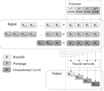
Fig. 2 The structure of GroundWater Artificial Neural Net- work (GWANN) model used in the study
production among wellfields is rotated based on projected groundwater levels at specific locations currently using artificial neural network models (i.e., GWANN model).
Originally Integrated Surface and Ground-Water (ISGW) model that couples hydrologic simulation programs for surface and subsurface system was used for the OROP. The current stochastic GWANN model was considered to overcome the limitation of the deterministic modeling system, ISGW such as the deficiency of spatial resolution and spin-up simulation
for numerical stability.
The GWANN model currently generates 1-week to 4-week forecasts of groundwater levels at 54 monitoring wells using recent observed rainfall, pumping and groundwater levels, and a rainfall forecast that assumes that the same rainfall observed in the week prior to the forecast will occur over the next 4 weeks (Fig. 2). Meanwhile, various usable climate data (i.e., short/long-term rainfall forecasts) are currently available to improve hydrologic forecast and TBW has been trying to employ such a forecast data for their operation system. It may be essential to examine sensitivity of climate inputs (i.e., rainfall in this study) to existing system and to assess the benefits of incorporating seasonal rainfall forecasts into water planning process.
The objective of this study is to examine how reliability can be improved, or risk can be reduced, by incorporating seasonal climate forecasts into the TBW resource planning processes that forecasts both supply and demand of the region for the upcoming weeks. This paper introduces the GWANN model that TBW developed for short-term water supply planning in Tampa Bay region and the framework to evaluate the model sensitivity of climate forcing. In this study, several hypothetical rainfall forecasts (i.e., percentiles of historic observation (i.e., climatology), real weekly observation, etc.) were applied for current GWANN model to 1 to 4-week forecast groundwater level and the GWANN model outputs using the weekly rainfall scenarios were evaluated comparing to observed groundwater level data.
II. STUDY AREA AND DATA
1. Target stations
As described above, Florida's aquifers vary in depth, composition, and location, and are divided into two general categories: Surficial and Floridan. Surficial aquifers are separated from the Floridan aquifer from a confining bed of soil. In surficial aquifers, the groundwater continuously moves along the hydraulic gradient from areas of recharge to places of discharge. Surficial aquifers are recharged locally as the water-table fluctuates in response to drought or rainfall. The Floridan aquifer, in contrast to surficial aquifers, is the portion of the principal artesian aquifer that
Table 1 Aquifer classification for monitoring wells used in the study
Wellfield Name
Well Name
Aquifer Group
Wellfield Name
Well Name
Aquifer Group CBR
SRWs W
MRB
SGW1sAR W
SERWs W MB4s W
A1s W MB23s W
COS
Keystone36 W MB24s W
JAMES10s W MB537s W
COS20s W MB25s W
Calm33A -
NOP
NPMW7s W
James11d F NPMW8s W
Cosme3 F NPMW9s W
CYB
WT2_500 W
S21
HILLS13s W
WT5_200 W JCKSN26s W
WT9_500 W HILLS13d F
WT2_1000 W JCKSN26d F
CYC
TB22sAR W Lutzpk40s W
TMR1As W
SOP
NORTHs W
TMR2sR W SP47s W
TMR4sAR W HARRYMs W
TMR1d F SR54d F
TMR2d F SP42d F
TMR3d F SP45d F
TMR4d F
STK
STK20s W
TMR5d F SM2s W
EDW
SM28ARs W EMW16s W
EW11ARs W EMW08s W
SM15ARs W WT15s W
EW2Sdp -
F: Floridan aquifer W: Surficial aquifer - : not identified
EW139G -
EW113B -
EW2N unknown
extends into Florida. In this study, 54 monitoring wells are selected for model evaluation and those are classified by the aquifer type as shown in Table 1. Then the results were evaluated for each well and method separately because the model performance for each well type may be different.
These monitoring wells are located at major production wellfields (Fig. 1) of which data have been used as control points to optimize operation plan (i.e., OROP) for water supply.
2. Data
Historical rainfall data are retrieved directly from the enterprise web database (http://gis.tampabaywater.org/rainfall/)
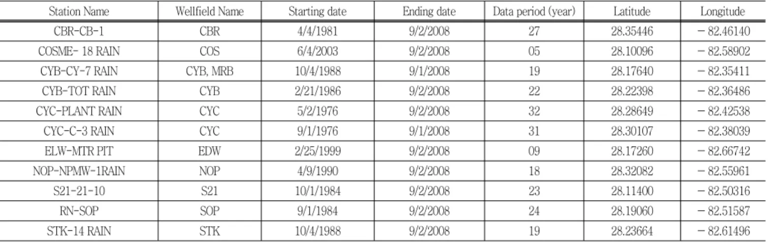
Table 2 Rainfall stations and data information
Station Name Wellfield Name Starting date Ending date Data period (year) Latitude Longitude
CBR-CB-1 CBR 4/4/1981 9/2/2008 27 28.35446 -82.46140
COSME- 18 RAIN COS 6/4/2003 9/2/2008 05 28.10096 -82.58902
CYB-CY-7 RAIN CYB, MRB 10/4/1988 9/1/2008 19 28.17640 -82.35411
CYB-TOT RAIN CYB 2/21/1986 9/2/2008 22 28.22398 -82.36486
CYC-PLANT RAIN CYC 5/2/1976 9/2/2008 32 28.28649 -82.42538
CYC-C-3 RAIN CYC 9/1/1976 9/1/2008 31 28.30107 -82.38039
ELW-MTR PIT EDW 2/25/1999 9/2/2008 09 28.17260 -82.66742
NOP-NPMW-1RAIN NOP 4/9/1990 9/2/2008 18 28.32082 -82.55961
S21-21-10 S21 10/1/1984 9/2/2008 23 28.11400 -82.50316
RN-SOP SOP 9/1/1984 9/2/2008 24 28.19060 -82.51587
STK-14 RAIN STK 10/4/1988 9/2/2008 19 28.23664 -82.61496
maintained by TBW. The pumpage and groundwater level for the monitoring wells distributed in each wellfield over the study area (Fig. 1) were collected from TBW. Rainfall station data located near each wellfiled are used to generate statistical percentile forecast and data period and corresponding wellfields are listed in Table 2. Because the experiments for the study were conducted for 2 years from 2006 to 2007, the observation data since the end of 2005 were used in the study.
III. METHODOLOGY
1. GWANN model
A. Background
Artificial Neural Networks (ANN) have been widely used for a number of reasons/cases 1) where the underlying process to be modeled is not well known prior, 2) when there is no enough data to support a physically based or models; or 3) when using physically based process model is too expensive to computationally run such as the case demonstrated here. The main advantage of using ANN is that multiple simulations (e.g., surface and subsurface system) at a specific point location can be provided in a more effective way of modeling without explicitly accounting for the underlying physical process governing the flow of water. ASCE (2000a and 2000b) summarizes ANN applications in hydrology and lists some of the advantages and disadvantages of using them. In the past decade, there has been a growing number of ANN for estimating groundwater
levels. Johnson and Rogers (2000) used ANNs to substitute time-consuming flow and transport models in a hypothetical case study on optimizing remediation in ground water.
Coulibaly et al. (2001) used four types of ANN models to predict monthly shallow ground-water table fluctuations and reported that ANNs provided accurate prediction when data are too scarce to run a physically based model.
Coppola et al. (2003) developed ANN models to predict transient ground-water levels at 12 monitoring locations and concluded that the ANN-predicted ground-water levels were better than predictions from the calibrated numerical model. Asefa et al. (2007) compared the performance of three ANNs (Feed Forward Back Propagation (FFBP), Radial Basis Network (RBN), and Generalized Regression Networks (GRN) to forecast groundwater levels up to four week in advance and concluded that even though the FFBP networks require relatively high computational costs, they were the most accurate models of the three. These models are currently implemented in GWANN model and are used on near real-time basis.
B. Model structure
Details of GWANN model development (training and testing) is documented in Asefa et al. (2007). The model is developed based on a water balance concept where groundwater level is modeled as a function of initial heads, boundary conditions, and changes in stresses (rainfall and pumpage) at weekly time scale and is briefly summarized as following. Groundwater level was forecasted for weeks 1 through 4 as
Ⅰ (1)
Where is groundwater level to be forecasted for week i, Ⅰ is the Feed Foreward Back Propagation (FFBP) function that was estimated by training, and Ⅰ is the vector of input which has the following form:
Ⅰ (2)
Where P, WL, and Q represent precipitation, groundwater level that are boundary conditions (e.g., lakes), and pumpage, respectively. The subscript represents the extent of past initial conditions that are used in the model. Fig. 2 sche- matically represents the structure of GWANN model. The models were trained using repeated training resampling as wells as random initial weight in order to avoid and possibility of the optimization to be restricted to a local optima, which is a drawback of ANNs
2. Hypothetical rainfall scenarios
In order to investigate to what extent, improved rainfall forecasts may improve weekly and monthly model predictions of groundwater levels, we consider various weekly rainfall forecasts (historic period of record percentiles (20th, 50th,
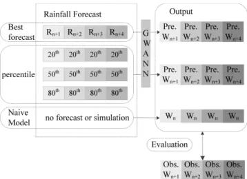
Fig. 3 Schematic representation of the alternative forecast scenarios: ‘best forecast’, ‘percentile forecast’, and the conceptual ‘naïve model’ (which assumes ground- water levels for the next four weeks will be equal to the previous week's groundwater level)
and 80th) and the “best” forecast (using the actual observed rainfall). The GWANN model results using these scenarios were compared to naïve model performance. Naïve model is referred as the conceptual model which assumes ground- water levels for the next four weeks will be equal to the previous week's groundwater level. Fig. 3 is a schematic representation of the alternative forecast scenarios used in this study (i.e., the ‘best forecast’, ‘percentile forecast’, and ‘naïve model’).
3. Error statistics
Root mean square error statistics (Eq. 3) and Theil's U statistics (Eq. 4) were used to quantify the accuracy of the groundwater level prediction using each method of rainfall forecast and the naïve model over the study period.
SE Nt N
t (3)
Where, N is the number of observations and
.
′
∑ ′′
∑ ′
(4)
Where, ′ and ′
The Theil's U (TU) measures to what extent the results are better than those of a naïve or trivial prediction. This coefficient makes it possible to analyze the quality of a forecast in the following manner:
- when U>1, the error in the model is higher than the naïve model error.
- when U<1, the error in the model is lower than the naïve error (good forecast); the lower coefficient (but≥
0) indicates the better forecast.
IV. RESULTS AND DISCUSSIONS
To develop the hypothetical rainfall forecasts, 20th, 50th, and 80th percentiles of weekly rainfall series for each 52
Fig. 4 Weekly total rainfall time series for the observations used in this study. The bright and dark gray zones represent total data range and 20th and 80th percentile of observation indicating the spatial variability of observed weekly rainfall over the 11 stations
Fig. 5 1st Week (first column) and 4th week (second column) groundwater level forecast results using each rainfall forecast for a surficial aquifer well, STK_WT15s (upper row) and a Floridan aquifer well, CYC_TMR2d (bottom)
starting week were calculated using the historic period of record. Fig. 4 shows the observed weekly rainfall time series for the study period over the 11 stations listed in Table 2. The figure denotes the strong seasonality with high rainfall during summer from June to September and dry season through the rest of period, and significant spatial variability of rainfall over the study area. Note that the percentiles represented in the figure indicate the spatial variation of actual rainfall sequences over the study domain and different than the climatology, which this study used as rainfall forecast (Fig. 3). Annual total rainfall amounts for the study years, 2006 and 2007 are 1259 mm
and 1204 mm, respectively.
Fig. 5 compares the results of the 1-week and 4-week ahead groundwater level (or the depth to the water table) forecasts using each method for a surficial (WT15s well in the STK wellfield) and Florida aquifer well (TMR2d well in the CYC wellfield which showed relatively good skills) to the observations as the examples of the results. These figures indicate that the skills of 1-week forecast are generally better than those of 4-week forecast and the differences among the models with various climate forcing increases as forecasting period get longer.
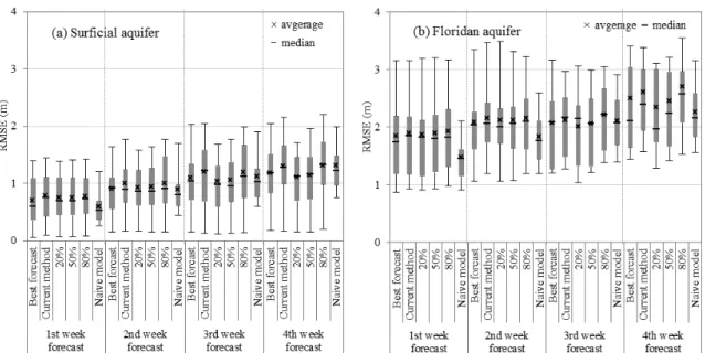
To quantitatively evaluate the results, RMSE of the
Fig. 6 Average root mean square error (RMSE) comparison of groundwater levels predicted using each rainfall forecast for (a) surficial aquifer wells and (b) Floridan aquifer wells over the study period
forecasts were compared in Fig. 6. The results indicate that using the actual weekly rainfall observation (i.e., ‘best forecast’) and using long-term 20th and median weekly rainfall (i.e., ‘20 %’ and ‘50 %’ in the figures) as the forecast, show better skills over using the current method. While for the 1 and 2-week ahead forecasts, the sensitivity of model forecasts to the rainfall forcing and model skills (comparing to naïve model) appears to be inconsiderable, the benefits of using the ‘best forecast’ were prominent for the 3 and 4-week ahead forecasts. As the forecasting period increases from 1-week through 4-week, RMSE tends to increase by the rate of 0.2 m/ week. For the surficial wells, the results showed lower RMSE, reduced by 0.1 m to 0.2 m for the 1-week forecast, and 0.1 m to 0.3 m for the 4-week forecast comparing to Floridan aquifer wells.
The results for Floridan aquifer wells, in general showed larger RMSE ranging from 0.9 m to 3.6m. It is likely because several Floridan aquifer wells (e.g., CBR and CYC wellfields) showed unusual/poor behavior. The poor predictions of several Floridan wells, which contributed to the higher RMSE may have resulted from the short data period used for evaluation (only two years tested here) compared to several years of data that was used to test and validate the models. Also, note that the model structure calls for eight weeks of initialization from rainfall, 13 weeks from
pumpage and 4 weeks for boundary conditions. The data used for the test and validation were not used here because the objective of the study is an assessment of performance using independent forecast data. Additionally the model would possibly be less skillful for the underlying confined system because of sharp fluctuation which results from the water management (i.e., pumping) and slow recovery rate (Fig. 5).
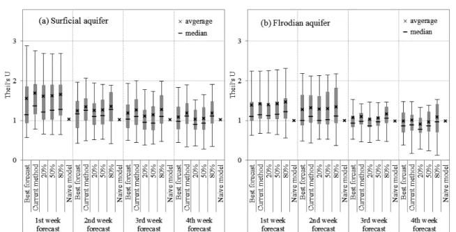
Fig. 7 compares the TU statistics for each forecast and naïve model (recall that theoretically TU for naïve model is 1). The results consistently show that ‘best rainfall forecast’ and 20th and 50th percentile of climatology generally improves forecast skills over the current method by 4 % (1-week forecast) to 9 % (4-week forecast) for the study period. It is likely because the two year rainfall data used here happen to be within 20th and 50th of the historical data. The averaged TU statistics of 1-week ahead forecasts for the surficial aquifer ranges from 1.55 (best forecast) to 1.68 (current method). For the Floridan aquifer, TU statistics for the best forecast and the current method were 1.39 and 1.42, respectively. These results indicate that the best rainfall forecast improves model performance over the current method, regardless of the aquifer where the monitoring wells were located. Note that the TU statistic for the surficial aquifer is generally higher (poorer performance) than for
Fig. 7 Theil's U statistics comparison of groundwater levels predicted using each rainfall forecast for (a) surficial aquifer wells and (b) Floridan aquifer wells over the study period
the Floridan aquifer because the naïve model provided better forecasts for the surficial aquifer compared to the Floridan aquifer that is, change rate of weekly groundwater level and error of naïve forecast for surficial aquifer is less than that of Floridan aquifer as shown in Fig. 6.
Especially for 3 and 4-week ahead forecasts, the results using 50th percentile of historical rainfall showed as similar skills to the current method and 80th percentile results were slightly worth than the current method for the Floridan aquifer. Comparing to naïve model, for more than half of surficial aquifer wells the model forecasts were worth than naïve model even for 4-week ahead forecast (Fig. 7a). In contrast, the median TU statistics of the 3 and 4-week forecasts for floridan aquifer were less than 1, which indicates the potential utility of rainfall forecasts including the current method for many wells.
However, for the rest of wells (especially in surficial aquifer wellfield), TU measures for the GWANN results using any methods were greater than 1 for 1 thorough 4-week forecasts indicating that naïve model forecast give better prediction than the GWANN model using any rainfall forecasts. RMSE comparison results showed that 1 to 2-week old groundwater level could be reliably used as forecast instead other rainfall forecast scenarios under the current forecast system while more accurate rainfall
forecast improved 3 to 4-week forecast.
Overall, model results indicated that using a best rainfall forecast and lower percentile of weekly climatology (e.g., 20th~50th) as the forecast for each of the next 4 weeks modestly reduced model prediction error over using the current method. The comparison of the results using various weekly rainfall forecasts denoted that the GWANN model performance could be improved by employing the better rainfall forecasts. While the GWANN model is not likely sensitive to rainfall forecasts for the first two weeks' forecasts with insignificant differences among the different rainfall forecasts, the model forecasts showed meaningful sensitivity to rainfall forcing and better skill for 3 and 4-weeks forecasts compared to the naïve model results (for more than half of wells).
V. CONCLUSION
This study investigated the utility of improved rainfall forecast in current groundwater level forecasting tools and water resources managements in west central Florida. The current groundwater level forecasting model (GWANN) in TBW uses recent observed rainfall, pumping and groundwater levels, and a rainfall data for the weeks prior to the forecast period as input forecasts. Employing a reliable climate
forecast may improve the model performance. In order to demonstrate, to what extent improved rainfall forecasts may improve weekly model predictions of groundwater levels, we suggested various rainfall forecasts (historic period of record percentiles (20th, 50th, and 80th), and the ‘best forecasts’ (observed rainfall)).
The results indicate that using the ‘best forecast’ and 20th percentile and median of the long-term climatology as the rainfall forecast improves the skills of groundwater level forecasts over the current method for the study period. Comparisons of the forecast results and naïve model results indicate that skills of forecasts even using the ‘best forecast’ appeared to be better than using historical constants (i.e., naïve model) for more than 3-week ahead. Additionally, using the actual observed rainfall reduced the errors of groundwater level forecasts over the current method but not prominent improvement over the forecasts using historical percentiles or current method.
These indicate that accurate climate forecasts would be of benefit to the monthly forecast in water supply operation system, however in order to substantially utilize high quality climate information (if any) the current modeling system need to be further improved for the specific wells of interest.
It should be also noted that the skills of GWANN model results using various climate scenarios vary to application region and training period as well. That is, the structural enhancement of the GWANN, such as retraining the neural networks using forecast rainfall or other forecast climate indices; or extending the forecast/planning horizon beyond four weeks may be necessary prior to employing improved rainfall forecasts. The applicability of the results drawn in this study would be limited by the small sample size (two years) and thus a rigorous investigation with more data is recommended to derive concrete conclusions.
REFERENCES
1. ASCE task committee on application of artificial neural networks in hydrology (Rao Govindaraju), 2000a.
Artificial Neural Networks in Hydrology. I: Preliminary Concepts. ASCE Journal of Hydrologic Engineering 5(2): 115.
2. ASCE task committee on application of artificial neural networks in hydrology (Rao Govindaraju), 2000b.
Artificial Neural Networks in Hydrology. II: Hydrologic Applications. ASCE Journal of Hydrologic Engineering 5(2): 124-137.
3. Asefa, T., N. Wanakule, and A. Adams, 2007. Field-scale application of three types of neural networks to predict groundwater levels. Journal of the American Water Resources Association 43(5): 1245-1256.
4. Coppola, E., F. Szidarovszky, M. Poulton, and E.
Charles, 2003. Artificial neural network approach for predicting transient water levels in a multilayered groundwater system under variable state, pumping, and climate conditions. Journal of Hydrologic Engineering 8(6): 348-360.
5. Coulibaly, P., F. Anctil, R. Aravena, and B. Bobee, 2001. Artificial neural network modeling of water table depth fluctuations. Water Resources Research 37(4):
885-896.
6. Hwang, S., 2012. Utility of gridded observations for statistical bias-correction of climate model outputs and its hydrologic implication over west central Florida.
Journal of the Korean Scociety of Agricultural Engineers 54(5): 91-102.
7. Hwang, S., C. Martinez, and T. Asefa, 2012. Assessing the benefites of incorporating rainfall forecasts into monthly flow forecast system of Tampa Bay Water, Florida. Journal of the Korean Society of Agricultural Engineers 54(4): 127-135.
8. Johnson, V. M. and L. L. Rogers, 2000. Accuracy of neural network approximators in simulation-optimization.
Journal Water Resources Planning and Management 126(2): 48-56.