ISSN 1225-0988 | EISSN 2234-6457 <Original Research Paper>
A Simulation Based Study on Increasing Production Capacity in a Crankshaft Line Considering Limited Budget and Space
Guan Wang
1․Shou Song
1․Yang Woo Shin
2․Dug Hee Moon
1†*1
Department of Industrial and Systems Engineering, Changwon National University
2
Department of Statistics, Changwon National University
예산과 공간 제약하에서 크랭크샤프트 생산라인의 생산능력 증대를 위한 시뮬레이션 기반의 연구
왕 관
1․송 수
1․신양우
2․문덕희
11
창원대학교 산업시스템공학과 /
2창원대학교 통계학과
In this paper, we discussed a problem for improving the throughput of a crankshaft manufacturing line in an automotive factory in which the budget for purchasing new machines and installing additional buffers is limited.
We also considered the constraint of available space for both of machine and buffer. Although this problem seems like a kind of buffer allocation problem, it is different from buffer allocation problem because additional machines are also considered. Thus, it is not easy to calculate the throughput by mathematical model, and therefore simulation model was developed using ARENA
®for estimating throughput. To determine the inves- tment plan, a modified Arrow Assignment Rule under some constraints was suggested and it was applied to the real case.
Keywords: Production Capacity, Crankshaft Line, Limited Budget and Space, Modified Arrow Assignment Rule, Simulation
1. Introduction
The major components that make up an engine are popularly called the 5C’s, namely, camshaft, crankshaft, cylinder block, cylinder head, and connecting rod. These major components are machined and assembled in their respective manufactur- ing sub-lines, and the completed components are transferred to the final engine assembly line. A final engine assembly line then consists of a series of assembly operations (Xu et al., 2012).
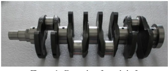
A crankshaft is the part of engine that changes the recip- rocating linear piston motion into the rotation motion (see
<Figure 1>). To produce a crankshaft, various machining processes such as milling, drilling, turning, rolling, grinding, finishing, burnishing, and measuring processes are required.
Although the process-flow of a crankshaft line is different among automotive factories, the typical layout concept is the flow-line having multiple parallel machines.
In general, the production lines of the components of an engine are highly automated. However, there are many rea- sons which could cause the breakdown in a process, and they
This research was partially supported by the Basic Research Program through the National Research Foundation of Korea(NRF), funded by the Ministry of Education(Grant Number NRF-2013R1A1A2058943 and NRF-2012R1A1B3004158).
†Corresponding author : Professor Dug Hee Moon, Department of Industrial and Systems Engineering, Changwon National University,
Gyeongnam, 641-773, Korea, Tel : +82-55-213-3723, Fax : +82-55-266-4464, E-mail : [email protected]
Received March 21, 2014; Revision Received April 21, 2014; Accepted May 29, 2014.
are machine failure, changing tools, repair parts, set-up change, and so on. Some of these events occur with deterministic in- terval, but others occur with stochastic interval. Thus, buffer is installed between two successive operations to reduce the effects of starvation and blockage. The uncertainty of the breakdown influences the performance of the line, and it is also the main reason why most automotive factories imple- ment a computer simulation to verify the layout design.
Figure 1. Example of crankshaft
There have been some researches using simulation that dealt with the design problem of a production line in an auto- motive factory. Since the whole system was too complicated, most of the studies in literature focused on the individual shop such as body shop, paint shop, engine shop, transmis- sion shop and general assembly shop. Ulgen et al. (1994) dis- cussed how to use of discrete-event simulation in the design and operation of body and paint shops, and they classified the use of simulation in the body shop into two aspects. The first classification was based on the stage of development of the system and the second was based on the nature of the problem investigated.
Jayaraman and Agarwal (1996) addressed a general con- cept when the simulation technique is applied to the engine plant, and Jayaraman and Gunal (1997) presented a simu- lation study in a testing area of an engine plant. The simu- lation studies regarding the engine block line have been sug- gested by Choi et al. (2002), Kumar and Houshyar (2002). In Moon et al. (2003), they considered the tool change times for specialized machines not equipping ATC (Automatic Tool Changer) in an engine block line. Dunbar III et al. (2009) de- scribed the simulation study of alternatives for transmission plant assembly line. Xu et al. (2010) compared three differ- ent types of layouts in automotive engine block lines and Moon et al. (2012) analyzed the effect of failure distribution in automotive engine line. Xu et al. (2012) presented a case study that integrates a simulation study with Analytic Hierar- chy Process (AHP), and the integrated model was applied to the design of a transmission case line in a Korean automotive factory. The process-flow of the engine block line is similar to that of the crankshaft line or transmission case line.
The crankshaft line considered in this paper is an existing
system operated by a Korean automotive company. The fac- tory has a plan to increase the production capacity within the limited budget to meet the increasing demand, and thus, it is necessary to find where is the bottleneck for growing up throughput.
There have been some researches which deal how to find bottlenecks in manufacturing systems for improving the per- formances of systems (see Li and Meerkov, 2009; Lawrence and Buss, 1994; Kwon and Lim, 2013; Li et al., 2011). Most of the papers have focused on developing the detecting meth- ods for bottlenecks.
Another area related to this paper is buffer allocation problem. There have been many researches dealing with the optimal buffer allocation problem. Powell (1994) studied the buffer allocation problem for unbalanced lines with three machines. Rules of thumb for the optimal sequential place- ment of buffer space were developed. Seong et al. (1995) used gradient search algorithm when the objective function is to maximize net profit. So (1997) presented a study on the optimal buffer allocation problem of minimizing the average work in process subject to a minimum required throughput and a constraint on the total buffer space. Gershwin and Schor (2000) suggested primal-dual problem considering optimal buffer space allocation in a serial line. A primal problem minimized total buffer space subject to a production rate con- straint, and a dual problem maximized production rate sub- ject to a total buffer space constraint. However, they did not consider the profit including cost. Huang et al. (2002) con- sider a flow shop-type production system and use a dynamic programming approach to maximize its production rate or minimized its work in process under a certain buffer alloca- tion strategy. Chan and Ng (2002) compared buffer alloca- tion strategies for maximized the production rate in serial production line. Amiri and Mohtashami (2012) presented a multi-objective formulation of the buffer allocation problem in a serial line in which unreliable machines, finite buffer and exponential service time were assumed. They developed a meta-model for estimating production rate based on discrete event simulation, and used genetic algorithm combined to line search method to solve the multi-objective model, max- imizing production rate and minimizing buffer size, and de- termining the optimal (or near optimal) size of each buffer storage.
In this paper, we combine the simulation study for ana-
lysing manufacturing system and the bottleneck search meth-
od to determine investment plan considering the limitation of
budget and available spaces for machines and buffers. The
configuration of the crankshaft line and the mathematical
model for optimizing investment plan under the limits of bud-
get and available space are described in section 2. In section 3,
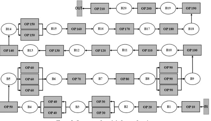
Figure 2. Processes of crankshaft manufacturing Table 1. Descriptions of operations
OP No Processes Number of
Machines(As-Is) Cycle Time
(sec.) Machine Price
($1,000) Extra Available Spaces
OP-10 Mass Centering 1 50 1,180 0
OP-20 Rear Turning 1 46 230 0
OP-30 Rough JR/Pin Milling 2 140 952 1
OP-40 Journal Grooving 2 152 1,012 1
OP-50 Pin Grooving and Milling 1 50 962 0
OP-60 Oil Hole Drilling 3 195 357 2
OP-70 Middle Washing 1 48 120 0
OP-80 Deep Rolling 1 51 1,010 0
OP-90 Re-centering and Hole Drilling 3 198 357 2
OP-100 Trust Turn and Rolling 1 48 270 1
OP-110 Journal Head Grinding 1 75 833 1
OP-120 Orbital Pin Grinding 1 52 1,190 1
OP-130 Front Angular Grinding 1 47 476 1
OP-140 Rear Angular Grinding 1 54 476 1
OP-150 CPS Hole Boring 2 160 417 2
OP-160 Final Balancing 1 48 726 0
OP-170 Deburring 1 48 350 0
OP-180 Lapping 1 50 500 0
OP-190 Final Washing 1 48 370 0
OP-200 Final Measuring 1 50 350 0
OP-210 Sprocket Assembly 1 51 390 0
simulation model is introduced and modified arrow assign rule for finding the best investment plan is suggested. The re- sult of case study and its optimality are explained in section 4, and conclusion and further study are discussed in section 5.
2. Configurations and Objective
The layout concept of the crankshaft line considered in this paper is a typical flow line as shown in <Figure 2>. In order to enhance the ease of machining or to reduce the risk of the breakdown of a line, some operations have two or three iden- tical machines in parallel where a part chooses only one of machines and then it goes to the next operation after opera- tion. Here, OP-30, OP-40, OP-60, OP-90 and OP-150 consist of multiple identical machines in parallel.
We assume that only one type of crankshaft is produced in this line, and the target of annual production quantity is 120,000 units. The annual working days are 261 days (21.75 days per month) and the working hours are 10 hours per day including the two hours of overtime.
2.1 Configurations of the System
• Operations and Cycle Times
Operations are designed considering the types of processes and the target tact time. If there are no failure, no tool change, no starvation and no blocking, the ideal target tack time is 261×10×3600/120,000 = 78.3 seconds. <Table 1> shows the details of operations including number of machines and oper- ation cycle time. The longest average cycle time of an oper- ation is 80 seconds at OP-150 when we assume that there are two machines in OP-150. Thus, this factory has to reduce the cycle times of some operations to meet the target production quantity.
At each operation, we assume that operation cycle time is deterministic because most of the machines are automated.
Loading and unloading times are included in the operation cycle time. In some operations, there are multiple parallel machines for one operation because the tasks are complex, and it is difficult to separate them into two operations. Fur- thermore, an operation is composed of more than one proc- ess, for example there are 16 drilling and milling processes in OP-60, and 16 types of tools and their life cycles should be considered for modeling.
This factory has been built with some extra machine spaces and buffer spaces in some operations that give a possibility of making a plan to increase the throughput almost twice.
<Table 1> lists the existing number of machines, extra avail-
able space, cycle time and machine price for each operation.
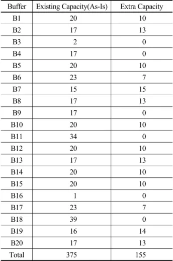
Table 2. Buffer capacity
Buffer Existing Capacity(As-Is) Extra Capacity
B1 20 10
B2 17 13
B3 2 0
B4 17 0
B5 20 10
B6 23 7
B7 15 15
B8 17 13
B9 17 0
B10 20 10
B11 34 0
B12 20 10
B13 17 13
B14 20 10
B15 20 10
B16 1 0
B17 23 7
B18 39 0
B19 16 14
B20 17 13
Total 375 155
• Buffers
Various types of conveyor are used in the line for trans- portation and storage. A part should be loaded on a jig for transportation. Thus, the buffer capacity listed in <Table 2>, means the maximum number of jigs to be installed in a con- veyor between two successive operations. In B3, B4, B9, B11, B16 and B18, there is no available space for additional buf- fer. The price of additional one buffer (jig) is $200, and the total investment cost for all additional buffers is $200×155 =
$31,000.
• Down Times
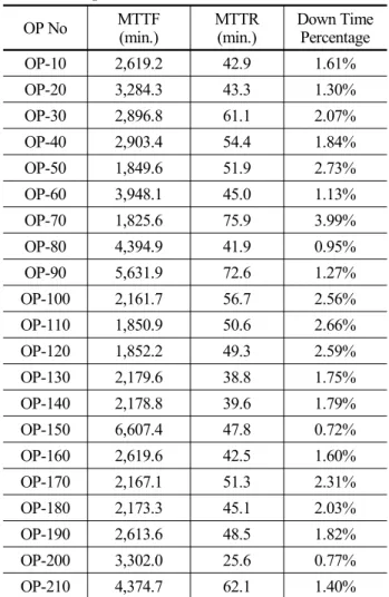
Two kinds of downtimes, machine failure and tool exchange are considered. The failure distributions are obtained from the historical data. The MTTF (Mean Time to Failure) and the MTTR (Mean Time to Repair) of the machine failure are list- ed in <Table 3>. The distribution functions of failure time and repair time are assumed to be exponential, and time de- pendent failure is assumed.
Tool change (or tip change) is assumed to be operation de-
pendent failure. That is, tool change (or tip change) is re- quired at every predetermined number of parts, and the num- ber is defined as MCBF (Mean Count between Failures). If there are two or more tools in a machine, the MCBF's of tools are independent and may be different from each other.
Most of machining centers equip ATC (Automatic Tool Changer) and many tools are inserted in tool magazine.
<Table 4> lists the tool types and MCBF of OP-90, where 14 tools are in ATC. Tool change time is the sum of the time for opening (and closing) door, the time for exchange tool and the time for in-line gauging. Opening and in-line gauging times are constant which are given as
∘ Time for opening and closing door = 0.33 minutes,
∘ Time for in-line gauging = 3 minutes.
The time for exchange tools depends on the number of tools to be changed and it is given as
∘ Time for exchange tool = 0.67 minutes/tool.
Table 3. Input data of MTTF and MTTR
OP No MTTF
(min.) MTTR
(min.) Down Time Percentage
OP-10 2,619.2 42.9 1.61%
OP-20 3,284.3 43.3 1.30%
OP-30 2,896.8 61.1 2.07%
OP-40 2,903.4 54.4 1.84%
OP-50 1,849.6 51.9 2.73%
OP-60 3,948.1 45.0 1.13%
OP-70 1,825.6 75.9 3.99%
OP-80 4,394.9 41.9 0.95%
OP-90 5,631.9 72.6 1.27%
OP-100 2,161.7 56.7 2.56%
OP-110 1,850.9 50.6 2.66%
OP-120 1,852.2 49.3 2.59%
OP-130 2,179.6 38.8 1.75%
OP-140 2,178.8 39.6 1.79%
OP-150 6,607.4 47.8 0.72%
OP-160 2,619.6 42.5 1.60%
OP-170 2,167.1 51.3 2.31%
OP-180 2,173.3 45.1 2.03%
OP-190 2,613.6 48.5 1.82%
OP-200 3,302.0 25.6 0.77%
OP-210 4,374.7 62.1 1.40%
Since the tools having same MCBF should be changed at the same time, for example, T04 and T14 should be changed
in every 200 cycles, the tool changing time is 0.33+0.67× 2+
3 = 4.67 minutes. After producing 6,600 parts, six tools T04, T14, T01, T08, T09 and T02 should be changed at the same time, and the tool change time is 0.33+0.67×6+3 = 7.35 minutes.
• Defectives
Inspections for finding defectives are conducted in four operations OP-20, OP-50, OP-120 and OP-210, and the defect rates are 0.23%, 0.17%, 0.26% and 1.14%, respectively. We assume that there is no repair or rework for the defectives.
Table 4. Input data of tool changes (OP-90)
Tool No Tool Type MCBF
T04 TAP 200
T14 TAP 200
T01 DRILL 330
T08 REAMER 330
T09 DRILL 330
T12 END MILL 450
T13 DRILL 500
T07 DRILL 500
T02 INSERT TIP 660
T06 INSERT TIP 990
T11 INSERT TIP 1,350
T03 INSERT TIP 1,800
T10 TAP 2,000
T05 TAP 2,000
2.2 Objective of Study
The major concern of a company is to increase throughput within a limited budget. Generally, three types of strategies are usually applied to increase throughput, and they are buy- ing additional machines, installing additional buffers and re- placing tools with longer life cycles. However, in this paper we only consider the strategy of buying new machines and adding buffers. The total budget available is $1,050,000 and the prices of new machines and additional buffer are ad- dressed in section 2.1.
The mathematical model is defined as follows:
⋯
⋯
(1) s.t.
≤ , (2)
integer and ≤
≤
⋯ ,
integer and ≤
≤
⋯ ,
where
and
are the number of additional machines and its upper bound in operation i, respectively.
and
are the number of additional buffer and its upper bound be- tween operations i and i+1. Furthermore, is the throughput of the system,
is the price of machine I,
is the cost of additional one buffer and B is the total budget available.
3. Solution Procedure
3.1 Simulation Model
It is well known to be very difficult to derive analytical solution (i.e., approximation of queueing network) for the flow line with multiple unreliable machines, finite buffers, nonhomogeneous service times and the two types of failures.
Note that both of time dependent failure and operation de- pendent failure are included in the model and the failure dis- tribution functions are nonhomogeneous.
Simulation is known as useful tool for estimating the value of throughput ( ), WIP (Work In Process), starving proba- bilities and blocking probabilities at once. Simulation models were developed with ARENA
®(See Kelton et al. (2002)). To validate the simulation model developed, simulation run time was set to 146,410 minutes including 13,310 minutes of warm up time, and the number of replications was set to 100.
Then, the data gathering time was 133,100 minutes, and it was the 10 months in practice.
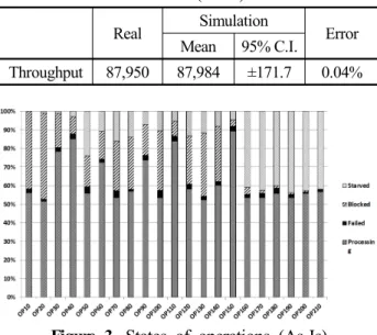
Table 5. Simulation result (As-Is) Real Simulation
Error Mean 95% C.I.
Throughput 87,950 87,984 ±171.7 0.04%
Figure 3. States of operations (As-Is)
The experimental results of 100 replications are presented in <Table 5>. The error obtained from simulation to the his- torical data in practice is 0.04%, and we conclude that the
simulation model is reasonably valid. The ratio of confidence interval to mean was 171.7÷87,984×100 = 0.2%. <Figure 3>
shows the portions of busy, idle (starvation), blockage and failure at each operation.
3.2 Modified Arrow Assignment Rule
The next step is to find which machine and buffer should be added to the existing system (As-Is) under the budget con- straint. If there are no constraints of budget, the possible number of investment plans (combinations) is
×
and that is about 3.61×10
18in this problem. If the additional assignment strategy of buffer is assumed to be just zero or full capacity, the number of investment plans is reduced to 5.66×10
7.
To solve the integer problem, various meta-heuristic algo- rithms such as genetic algorithm (GA), tabu search, gradient search and etc. can be used. In order to use GA, the fitness value, namely throughput (
), should be estimated for each chromosome. When the number of chromosomes in the first generation is set to 100, we need 100 simulation experiments.
If the number of the different chromosomes in the second generation is reduced to 70, we need additionally 70 simu- lation experiments. This process is repeated until the con- vergence is obtained. Furthermore, repair process is required for each crossover to consider the limited budget.
Similar situation is happened when various search algo- rithms are applied to this problem. Unfortunately, no meta- heuristic algorithms guarantee the global optimality, and it is the reason that why we need faster heuristic algorithm.
There are some algorithms to find the bottleneck in a flow line, e.g., ‘Arrow Assignment Rule’ (Li and Meerkov, 2009), and ‘Active Period Method’ (Lawrence and Buss, 1994; Kwon and Lim, 2013) and a method using autoregressive moving average (ARMA) model (Li et al., 2011). In Arrow Assign- ment Rule, they considered a serial line having only one ma- chine in each stage which has one type of time dependent failure, because they used mathematical approximation mod- el for estimating throughput, WIP, blocking probabilities and starving probabilities.
In this paper, we adopt the concept of Arrow Assignment Rule for finding bottleneck and modify it with the consid- erations of limited budget and extra spaces for machines and buffers. We also introduce the concept of investment effi- ciency as in equation (6) to find the priority of investment.
Denote by
and
the blocking probability of ma-
chine i (m
i) and the starving probability of m
iin steady state,
respectively and define the severity (
) of m
iby
⋯ , (3)
, (4)
. (5)
If
≥
, assign the arrow pointing from m
ito m
i+1. If
, assign the arrow pointing from m
i+1to m
i. In case that there are multiple machines with no emanating ar- rows, the one with the largest severity (
) is primary.
The following notations are used to explain the heuristic search rule. “Available” means that both of available space for machine (or buffer) and available investment cost are available. “Up” and “Down” means upstream and downstream, respectively. Efficiency is calculated by
. (6)
∘ TP : throughput,
∘ BN : set of bottleneck machines,
∘ COM : machine candidate,
∘ COB : buffer candidate,
∘ e(COM) : efficiency of machine COM
∘ e(COB) : efficiency of buffer COB
∘ p_BN_m : primary bottleneck machine having the largest
in BN,
∘ s_BN_m : set of secondary bottleneck machines having smaller
than p_BN_m in BN,
∘ s_BN_m_avl : subset of available machines in s_BN_m,
∘ s_BN_m* : machine having the largest
in s_BN_m_avl,
∘ p_BN_b : primary bottleneck buffer, where
≥
∘ s_BN_b : set of secondary bottleneck buffer related to each machine i in s_BN_m, where
≥
∘ s_BN_b_avl : subset of available buffers in s_BN_b,
∘ s_BN_b* : the buffer related to the machine having the largest
in s_BN_m,
∘
≥
∘ BN_side_m : set of machines on BN_side, which are not included in BN,
∘ BN_side_m_avl : subset of available machines in BN_
side_m,
∘ BN_side_m* : machine having the largest
in BN_side_
m_avl,
∘ BN_side_b : set of buffers on BN_side which are neither p_BN_b nor the buffers in s_BN_b,
∘ BN_side_b_avl : subset of available buffers in BN_side_b,
∘ BN_side_b* : the buffer related to the machine having the largest severity in BN_side_m,
∘
≥
∘ non BN_side_m : set of machines on non BN_side, which are not included in BN,
∘ non BN_side_m_avl : subset of available buffers in non BN_side_m,
∘ non BN_side_m* : machine having the largest
in non BN_side_m_avl,
∘ non BN_side_b : set of buffers on non BN_side which are neither p_BN_b nor buffers in s_BN_b,
∘ non BN_side_b_avl : subset of available buffers in non BN_side_b,
∘ non BN_side_b* : the buffer related to the machine having the largest
in non BN_side_m,
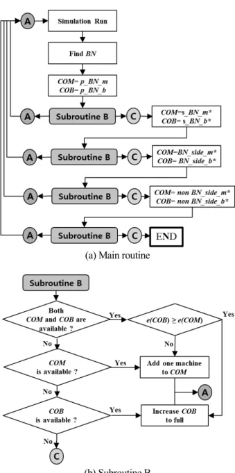
<Figure 4> explains the processes of search algorithm. The algorithm consists with a main routine and a subroutine B.
4. Case Study and Validation
4.1 Case Study
We carried out 100 replications of simulation run with the As-Is problem and the average throughput is 87,894. The set of bottleneck machines BN = {OP-40, OP-60, OP-110, OP- 150} is obtained as shown in <Figure 5>. Among the oper- ations in BN,
of OP-150 is the largest (
= 0.625), and thus p_BN_m is OP-150 and s_BN_m are OP-40, OP-60 and OP-110. Furthermore, p_BN_b is B14, because
, and s_BN_b are B4, B6 and B11 with respect to OP-40, OP-60 and OP-110. The upstream side of OP150 (p_BN_m) is BN side, and the downstream side of OP-150 is non BN side.
In the first round, the machine candidate (COM) is OP-150, because there are two extra available spaces, and the price of machine is $417,000 that is less than the total budget $1,050,000.
The buffer candidate (COB) is B14, because 10 extra buffers
are allowed and the cost of extra buffers is $2,000. Then, two
simulation experiments are carried out for the two cases (ad-
ding a machine to OP-150 and adding 10 buffers to B14) in-
dependently, and new simulation results including through-
put, WIP, starving probabilities and blocking probabilities
are obtained. The throughput after adding one machine in
OP-150 is 91,571 and the throughput in the case of increas-
ing the buffer B14 to full is 88,714. However, the investment
efficiency of the former is 8.6 and it is lower than 356 of the later. Thus B14 is selected to increased to full in the first round. The remaining budget is $1,048,000.
(a) Main routine
(b) Subroutine B
Figure 4. Flow chart of algorithm suggested In the second round, the elements in BN, p_BN_m and p_BN_b are the same as the first round except that COB (B14) becomes unavailable. Thus, one new machine is added to OP-150. The new throughput is 91,687 and the increment is 2973 units (3.35%). However, WIP decreases from 178.53 to 99.73.
In the third round, three operations (OP-40, OP-90 and OP-110) are included in BN, and OP-110 becomes p_BN_m and COM. But the machine price of OP-110 is higher than the remaining budget, $631,000, it is unavailable. Thus, we
increase the size of COB (B10) which is p_BN_b to full, and the throughput obtained from new simulation is 91,953, WIP is 98.49, and the remaining budget is $629,000.
In the fourth round, OP-110 is still p_BN_m, B10 is p_BN_b, OP-40 and OP-90 are elements of s_BN_m, and s_BN_b contains B4 and B8. However, both of COM and COB are unavailable since the remaining budget is not enough for adding a machine in OP-110 and B10 is already full. For the secondary bottlenecks, machine prices of OP-40 ($1,012,000) is over the remaining budget and there is no available space in B4. Thus, they are not in s_BN_m_avl and s_BN_b_avl., respectively and OP-90 becomes new COM and B8 becomes new COB. After simulations, e(COB) is 9.77 and e(COM) is 5.51. The next decision is to increase B8 to the full and then the new throughput is 92,121 and WIP is 99.63.
In the fifth round, OP-110 becomes p_BN_m. OP-40 and OP-90 are included in s_BN_m. s_BN_b contains B4 and B8.
By the logic, an additional machine is added to OP-90. Then, the throughput is increased to 92,551 and WIP is 105.12. The remaining budget is $269,400.
Figure 5. Candidates of bottleneck (As-Is)
The searching process is repeated until the remaining
budget is consumed completely. In the sixth round, there is
no available machine in p_BN_m, s_BN_m, BN_side_m, and
non BN_side_m, and no buffers are available in p_BN_b,
s_BN_b. Thus, we should check up BN_side first, and B2 is
selected as a COB and we increase the capacity of B2 to
maximum, because the severity of OP-20 is largest. Then the throughput becomes 92,611. Similarly, B6, B1, B5 and B7 are selected sequentially for COB in BN_side and their ca- pacities are increased to the upper bounds. After that, B19, B17, B15, B12, B13 and B20 are selected in sequence for COB in BN_side and their capacities are increased to the up- per bounds. Then the final throughput increases to 94,017 and WIP is 136.59. The total investment cost is $805,000 and the remaining budget is $245,000. The number of simulation experiments including As-Is analysis is 19 and the average simulation run time for each experiment is about 15 minutes.
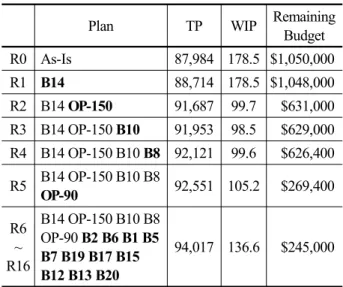
Table 6. Summary of solution processes
Plan TP WIP Remaining
Budget R0 As-Is 87,984 178.5 $1,050,000
R1 B14 88,714 178.5 $1,048,000
R2 B14 OP-150 91,687 99.7 $631,000 R3 B14 OP-150 B10 91,953 98.5 $629,000 R4 B14 OP-150 B10 B8 92,121 99.6 $626,400 R5 B14 OP-150 B10 B8
OP-90 92,551 105.2 $269,400 R6
~ R16
B14 OP-150 B10 B8 OP-90 B2 B6 B1 B5 B7 B19 B17 B15 B12 B13 B20
94,017 136.6 $245,000
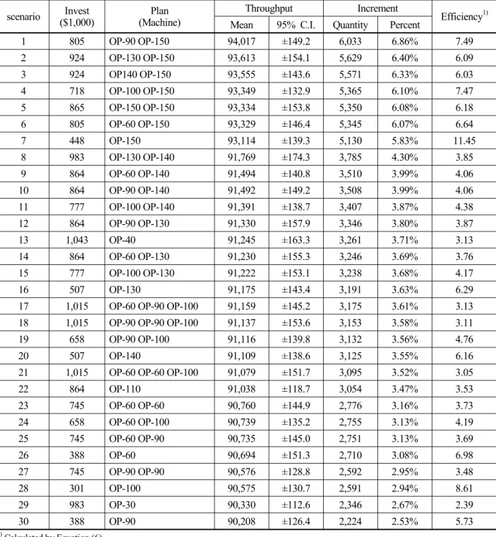
4.2 Validation for Optimality
To validate the solution procedure suggested, the best sol- ution obtained from section 4.1 is compared with the feasible solutions obtained from all enumerations. However the num- ber of all enumerations is too much big when we assume that the increment size of buffer is set to one. Thus, we inevitably assume that all available buffers are full, and search for the feasible investment plans for machines. Then the number of feasible plans is 30. If we assume that the capacities of some buffers remain without increasing, then the number of fea- sible plans must be greater than 30. <Table 7> lists the simu- lation results for all enumerations with the decreasing order of throughput, and scenario 1 is the best and it is the same to the investment plan that we obtained from our heuristic method.
5. Conclusions
In this paper, we discussed a simulation study for improving
the throughput of a crankshaft manufacturing line in an auto- motive factory, where there is the limitation of budget for purchasing new machines and installing additional buffers. In each operation and buffer, limited space is predetermined and it restricts the number of additional machines and buffers.
Although this problem seems like a buffer allocation prob- lem, it is not easy to calculate the objective function (throu- ghput) by mathematical model. Therefore, simulation model was developed using ARENA
®and the values of throughput, starving probabilities, blocking probabilities and WIP were obtained by simulation experiments.
To determine the investment plan, we modified arrow as- signment rule for considering parallel machines, the budget limitation and the space limitations of machines and buffers.
Then, the best solution by the modified arrow assignment rule was compared to the subset of all enumerations (30 cas- es), and the two results were same. Although the modified ar- row assignment rule does not guarantee the optimality, we obtained the best solution in the case study. Furthermore, the number of simulation experiments was reduced to 19.
The limitation of this paper is that we inevitably assumed that the buffer increment is nothing or full. However, this as- sumption can be relaxed such that the buffer increment is set to one. In this case, we can use the algorithm suggested with the slight modification of buffer increment size, but the num- ber of simulation experiments will be increased drastically.
For further research, the objective function can be changed to minimizing cost which includes investment cost and WIP cost. In this case the target throughput becomes new const- raint.
References
Amiri, M. and Mohtashami, A. (2012), Buffer Allocation in Unreliable Production Lines Based on Design of Experiments, Simulation, and Genetic Algorithm. International Journal of Advanced Manufactu- ring Technology, 62(1~4), 371-383.
Chan, F. T. S. and Ng, E. Y. H. (2002), Comparative Evaluations of Buffer Allocation Strategies in a Serial Production Line, Internatio- nal Journal of Advanced Manufacturing Technology, 19(11), 789- 800.
Choi, S. D., Kumar, A. R., and Houshyar, A. (2002), A Simulation Study of an Automotive Foundry Plant Manufacturing Engine Blocks, Proceedings of the 2002 Winter Simulation Conference, 1035-1040.
Dunbar, III, J. F., Liu, J. W. and Williams, E. D. (2009), Simulation of Alternatives for Transmission Plant Assembly Line, Proceedings of the Summer Computer Simulation Conference, 17-23.
Huang, M. G., Chang, P. L., and Chou, Y. C. (2002), Buffer Allocation in Flow-shop-type Production System with General Arrival and Ser- vice Patterns, Computers and Operations Research, 29(2), 103-121.
Jayaraman, A. and Agarwal A. (1996), Simulating an Engine Plant,
Table 7. Simulation results (all enumerations) scenario Invest
($1,000) Plan
(Machine)
Throughput Increment
Efficiency
1)Mean 95% C.I. Quantity Percent
1 805 OP-90 OP-150 94,017 ±149.2 6,033 6.86% 7.49
2 924 OP-130 OP-150 93,613 ±154.1 5,629 6.40% 6.09
3 924 OP140 OP-150 93,555 ±143.6 5,571 6.33% 6.03
4 718 OP-100 OP-150 93,349 ±132.9 5,365 6.10% 7.47
5 865 OP-150 OP-150 93,334 ±153.8 5,350 6.08% 6.18
6 805 OP-60 OP-150 93,329 ±146.4 5,345 6.07% 6.64
7 448 OP-150 93,114 ±139.3 5,130 5.83% 11.45
8 983 OP-130 OP-140 91,769 ±174.3 3,785 4.30% 3.85
9 864 OP-60 OP-140 91,494 ±140.8 3,510 3.99% 4.06
10 864 OP-90 OP-140 91,492 ±149.2 3,508 3.99% 4.06
11 777 OP-100 OP-140 91,391 ±138.7 3,407 3.87% 4.38
12 864 OP-90 OP-130 91,330 ±157.9 3,346 3.80% 3.87
13 1,043 OP-40 91,245 ±163.3 3,261 3.71% 3.13
14 864 OP-60 OP-130 91,230 ±155.3 3,246 3.69% 3.76
15 777 OP-100 OP-130 91,222 ±153.1 3,238 3.68% 4.17
16 507 OP-130 91,175 ±143.4 3,191 3.63% 6.29
17 1,015 OP-60 OP-90 OP-100 91,159 ±145.2 3,175 3.61% 3.13
18 1,015 OP-90 OP-90 OP-100 91,137 ±153.6 3,153 3.58% 3.11
19 658 OP-90 OP-100 91,116 ±139.8 3,132 3.56% 4.76
20 507 OP-140 91,109 ±138.6 3,125 3.55% 6.16
21 1,015 OP-60 OP-60 OP-100 91,079 ±151.7 3,095 3.52% 3.05
22 864 OP-110 91,038 ±118.7 3,054 3.47% 3.53
23 745 OP-60 OP-60 90,760 ±144.9 2,776 3.16% 3.73
24 658 OP-60 OP-100 90,739 ±135.2 2,755 3.13% 4.19
25 745 OP-60 OP-90 90,735 ±145.0 2,751 3.13% 3.69
26 388 OP-60 90,694 ±151.3 2,710 3.08% 6.98
27 745 OP-90 OP-90 90,576 ±128.8 2,592 2.95% 3.48
28 301 OP-100 90,575 ±130.7 2,591 2.94% 8.61
29 983 OP-30 90,330 ±112.6 2,346 2.67% 2.39
30 388 OP-90 90,208 ±126.4 2,224 2.53% 5.73
1)