IEG 환경지질연구정보센터

전체 글

(1)J. Soil Groundwater Environ. Vol. 24(5), p. 17~30, 2019. https://doi.org/10.7857/JSGE.2019.24.5.017 ISSN 1598-6438 (Print), ISSN 2287-8831 (Online). ≪ Research Paper ≫. MODFLOW-Farm Process Modeling for Determining Effects of Agricultural Activities on Groundwater Levels and Groundwater Recharge Kedir Mohammed Bushira1*·Jorge Ramírez Hernandez2 1. Corresponding author: Department of Water Resources and Irrigation Engineering, P. o. Box 21, Arba Minch University, Ethiopia 2 Instituto de Ingeniería, Universidad Autónoma de Baja California, Mexicali 21280, Baja California, Mexico. ABSTRACT Intensive agricultural development in Mexicali valley, Baja-California, Mexico, has induced tremendous strain on the limited water resources. Agricultural water consumption in the valley mainly relies on diversions of the Colorado River, but their water supply is far less than the demand. Hence, the use of groundwater for irrigation purposes has gained considerable attention. To account for these changes, it is important to evaluate surface water and groundwater conditions based on historical water use. This study identified the effects of agricultural activities on groundwater levels and groundwater recharge in the Mexicali valley (in irrigation unit 16) by a comprehensive MODFLOW Farm process (MFFMP) numerical modeling. The MF-FMP modeling results showed that the water table in the study area is drawn downed, more in eastern areas. The inflow-outflow analysis demonstrated that recharge to the aquifer occurs in response to agricultural supplies. In general, the model provides MF-FMP simulations of natural and anthropogenic components of the hydrologic cycle, the distribution and dynamics of supply and demand in the study area. Keywords : Mexico, MODFLOW farm process, Agriculture, Groundwater level, Groundwater recharge. billions of cubic meters of annual flow no longer reach, the. 1. Introduction. Gulf of California. This situation is largely driven by The determination of surface water and groundwater allo-. upstream diversions and economic forces that make the bor-. cations to farms is desirable for legal requirements (e.g.. der region one of the most productive geographic regions in. Stream volume adjudications), and for agro-economic deci-. México. This is also one of the driest regions in Mexico and. sion making ahead of the growing season. The need to. its explosive growth has put tremendous strain on the lim-. specify these flow rates applies to historic and future time. ited water resources. Agriculture in the Mexicali Valley. intervals (Schmid W. 2004). In Mexico groundwater already. withdraws approximately 2.5*109 m3 of water annually. represent 38% of total annual water withdrawal and agricul-. (Roman-Calleros and Ramírez-Hernández, 2003). Pumping. ture represents over three-fourths of the total groundwater. of groundwater for supplementary irrigation in the Valley. withdrawal at national levels.. has reduced groundwater levels significantly in some areas.. The Baja California-California border region is bounded. Increased groundwater use had induced leakage from rivers. by a common geography characterized by its booming pop-. and canals to groundwater, which has become the predom-. ulation, scarce water supply, and arid land. The natural riv-. inant form of surface water and groundwater interaction.. ers of this region are among the most regulated, used, and. Surface water and groundwater are highly connected due to. contaminated waterways in the world. These rivers are cur-. the sandy nature of the alluvial aquifer in the Valley.. rently used to the extent that they often no longer discharge. To help sustainably manage and conjunctively use these. to their respective termini, i.e. the Colorado River, whose. resources, there is needed to gain a better understanding of. *Corresponding author : [email protected]/[email protected] Received : 2019. 8. 16 Reviewed : 2019. 9. 2 Accepted : 2019. 10. 10 Discussion until : 2019. 12. 31 17.

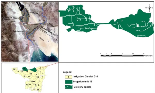
(2) 18. Kedir Mohammed Bushira·Jorge Ramírez Hernandez. Fig. 1. Location map of the study area (irrigation unit 16).. water movement in the hydrologic system through hydro-. 2. MF-FMP Features. logic modeling. MODFLOW Farm Process (MF-FMP) is a unique and. The Farm process (Schmid et al. 2006a, 2006b; Schmid. versatile alternative that provides fully coupled, cell-by-cell. and Hanson 2009a, 2009b) for MODFLOW-2005 (Har-. distributed fully iterative simulation of supply-constrained. baugh 2005) (MF-FMP) was developed to provide detailed. and demand-driven conjunctive use and movement of water. hydrologic budgets for all or part of a hydrologic system. from natural and anthropogenic sources.. and to examine how such budgets change over time. Con-. The alteration of the Colorado River delta of wilderness,. servation equations for groundwater, stream, lake, root. to the highly productive agricultural region that exists today. zone, and land-surface runoff processes are solved simulta-. in U.S.A-Mexico border region, brings many questions and. neously to simulate a large portion of the hydrologic cycle,. presents an excellent subject for a groundwater modeling. and the agronomic and human effects on the cycle. Among. study. How has the aquifer beneath the Colorado River. the mass conservation equations, the groundwater-flow. delta responded to the agricultural expansion when the Col-. equation (1) is the governing equation that is solved for. orado River water is changed from natural flow to sched-. groundwater heads.. uled releases? The main aim of this study was (1) to investigate the effects of agricultural activities on groundwater level and. ∂ ∂h ∂ ∂h ∂ ∂h ----- ⎛ Kh ------⎞ + ----- ⎛ Kh ------⎞ + ----- ⎛ Kv ------⎞ ±W = 0 ∂x ⎝ ∂x⎠ ∂y ⎝ ∂y⎠ ∂z ⎝ ∂z ⎠. (1). groundwater recharge and (2) to evaluate the sources of irri-. where h, is groundwater head (L), Kh and Kv are horizontal. gation water in user-defined water balance subregions. and vertical hydraulic conductivity (LT−1), respectively, W. (WBS) of commonly known by Irrigation Unit 16 (Fig. 1). is volumetric flux per unit volume representing sources and/. over 12 years using MODFLOW Farm Process (MF-FMP).. or sinks, x and y are horizontal co-ordinates (L), z is verti-. The stress packages in MF-FMP, among others, employed. cal co-ordinate (L) and t is time (T).. are; the Unsaturated Zone Flow (UZF1), Stream Flow Rout-. MF-FMP represents the components of evaporation and. ing (SFR), well package (WEL) and Drain package (DRN).. transpiration derived from precipitation, irrigation, and. J. Soil Groundwater Environ. Vol. 24(5), p. 17~30, 2019.

(3) MODFLOW-Farm Process Modeling for Determining Effects of Agricultural Activities on Groundwater Levels and Groundwater Recharge. groundwater on a cell-by-cell basis within user-defined. 19. runoff, given as time series data.. water-balance subregions (WBS). MF-FMP considers two. MF-FMP computes deep percolation (DP) as the sum of. types of water budgeting for the control volume horizon-. deep percolation below the root zone from precipitation and. tally delineated by land surface areas, called “farms”. These. irrigation, which can be instantaneous or delayed with link-. water-accounting units can include irrigated and non-irri-. age to the unsaturated zone infiltration package, UZF (Nis-. gated farms, native vegetation, and urban areas. Using the. wonger et al, 2006). It is the user-specified portion of losses. term “farm” in MF-FMP” has become somewhat of an. of precipitation and irrigation that are not consumptively. anachronism as MF-FMP has advanced to types of water-. used by plants and not lost to surface water runoff:. accounting units other than just agricultural farms. The water-accounting units in MF-FMP; do not include changes. p – loss. DP = ( P – ETp – act ) ( 1 – fr. I – loss. ) + ( I – ETi – act) ( 1 – fr. (6). in soil-water storage and, hence, are control interfaces at the land surface.. The current version of MF-FMP does not consider. For a given computational unit; a particular land use area in a given cell, the general mass-balance equation that MFFMP is based on for the root zone is the following: P. t+1. +I. t+1. t+1. t+1. + ETgw – act – ETc – act – R. t+1. – DP. t+1. changes in soil-water storage in the root zone (i.e., RHS in equation (2) = 0): P. t+1. t+1. t. θ –θ = ---------------------Δt. (2). and R. ). +I. t+1. t+1. t+1. + ETgw – act – ETc – act – R. t+1. – DP. t+1. =0. (7). MF-FMP still takes into account that the root zone might be inactive for conditions of wilting or anoxia. However, for any head between the lower and upper extinction depths,. t+1. t+1. t+1. (3). = R P + Ri. Where P is precipitation (LT−1), I is irrigation water (LT−1), −1. ETgw-act is root uptake from groundwater (LT ), ETc-act −1. is the total actual crop evapotranspiration (LT ), R is the −1. MF-FMP derives transpiration from groundwater; the residual crop water demand is then satisfied by transpiration from precipitation or irrigation. That is, at a steady state of soil moisture, ETc-act of equation (7) can be split into six components from three sources: groundwater, precipitation,. runoff from precipitation and irrigation (LT ), Rp is the. and irrigation (Tgw-act, Egw-act, Tp-act, Ep-act, Ti-act, Ei-. surface runoff from precipitation (LT−1), Ri is the irrigation. act,). All 6 components contribute to ETc-act However, Tp-. −1. surface return flow (LT ), DP is the deep percolation that −1. leaves the root zone as the moisture moves downward (LT ), t+1. θ. t. act, Ep-act, Ti-act, and Ei-act are outflows out of the landscape budget. In contrast, some parts of Tgw-act and Egw-. is the soil moisture at the end of a time step (L), θ is. act are inflows from GW into the root zone (landscape bud-. the soil moisture at the beginning of a time step (L), Δt is. get) but also outflows from the root zone into the atmo-. the time step length (T), and t is the time step index (dimen-. sphere.. sionless). MF-FMP computes R as the portion of crop-inefficient. 3. Materials and methods. losses from precipitation or irrigation that contribute to runoff:. 3.1. Study area p – loss. Rp = ( P – ETp – act )fr. (4). I – loss. Ri = ( I – ETI – act )fr. (5). Where, ETp-act and ETi-act are the portions of the ETc-act −1. fed by precipitation or irrigation (LT ), respectively, and p – loss. I – loss. of Mexico, bounded on the north by the State of California, USA, to the east by the State of Sonora, Mexico, to the west by the Pacific Ocean and south by the State of Baja California Sur (Fig. 1). Within the limits of the State of Baja California and. are fractions of the respective crop-. Sonora, is located the section of the Colorado River corre-. inefficient losses from precipitation or irrigation that go to a. sponding to Mexico, where the territorial boundary between. fr. and fr. The State of Baja California is located to the Northwest. J. Soil Groundwater Environ. Vol. 24(5), p. 17~30, 2019.

(4) 20. Kedir Mohammed Bushira·Jorge Ramírez Hernandez. the two States, which begins its journey in the dam diverter. ily urban land. Elevation in the study area ranges from. Jose Maria Morelos up reach the Gulf of California. The. about 41 m in the northeast to less than 5 m to south.. Colorado River Delta is one of the world’s largest deltas 2. The Mexicali Valley is characterized by a desert climate. covering over 8,600 km of terrain and extending across the. dominated by high temperatures and arid conditions. The. international border between the United States (U.S.) and. valley’s climate is defined by clear skies and plenty of sun-. the Republic of Mexico (Mexico). The Delta developed as a. light, with little precipitation given the atmospheric domi-. result of the constructive processes of sediment transport by. nance of high pressure. Average monthly high temperatures. the Colorado River and the destructive processes associated. in July are 42oC and the lowest average monthly high of. with, 1) the large tidal regime dominated by strong currents. 21oC occurs in December. The yearly average precipitation. in the upper Gulf of California and, 2) tectonic movement. is 72.5 mm, with monthly average precipitation values aver-. along the San Andreas Fault, which has transported sedi-. aging 0 mm in June and 12.4 mm in January.. ment NW across the Delta over millennia (Sykes 1935). Irrigation District 014 (Fig. 1) is divided into 22 irriga-. 3.2. Geology and Hydrogeology. tion units or irrigation administrative areas, for which. There are around five topographical areas in the Gulf of. pumping and irrigation data are aggregated and maintained. California: (1) the cutting edge subaerial Salton Trough, (2). by the National Water Commission of Mexico (CONA-. North Gulf Region, (3) Central Gulf Region, (4) South Gulf. GUA). The study area; the irrigation unit 16 (Fig. 1) ser-. Region, and (5) Gulf Mouth Region. During the Early to. vice areas encompass about 20,100 hectares, of which about. Middle Miocene (24 to 11 Ma), an earthbound volcanic. 85 percent is used for agriculture and, 15 percent is primar-. bend was shaped along what is currently generally the hub. Fig. 2. Geological map of the Baja California North. The study area is showed by an arrow in U.S.A Mexico border region. J. Soil Groundwater Environ. Vol. 24(5), p. 17~30, 2019.

(5) MODFLOW-Farm Process Modeling for Determining Effects of Agricultural Activities on Groundwater Levels and Groundwater Recharge. 21. of the advanced Gulf of California (Hausback 1984; Saw-. posed primarily of irregularly layered coarse gravel and. lan and Smith 1984). Those volcanic rocks comprise the. sand. This unit constitutes the main pathway for horizontal. storm cellar for the Gulf Extensional Province (Gastil et al.. groundwater flow in the system (Mock et al., 1988). Together. 1973). They make due as mountains made out of thick. the wedge zone and coarse gravel zone may represent what. andesite streams circumscribing the western side of the inlet. is described in research of the modeled Colorado river area. in peninsular Baja California (Fig. 2). More youthful volca-. area (i.e. Pacheco et al., 2006; Portugal et al. 2005; Chavez. nism began around 13 Ma in eastern Baja California and. et al. 1999; Barragan et al., 2001) as the upper sediments of. inside the creating Gulf of California crack. An examina-. the Mexican Colorado River delta basin with a composi-. tion of a multiple of well logs very near to the study area. tion of fluvial and alluvial not- consolidated sediments of. demonstrate that, there is unconsolidated irregular sequences. Pleistocene to Recent ages. Transmissivity values for the. of clay, sand, gravel and mud persist in area for at least 180. Wedge zone and Coarse Gravel zone combined were deter-. m below the land surface (Feinstein et al., 2008).. mined to range from 835 to 22,300 m2/day (Olmsted et al.. Soils in the valley are generally classified under the prin-. 1973). Horizontal hydraulic conductivity was calculated to. ciple soil order of Aridisols, according to the soil taxonomy. range up to 400 m/day. Vertical hydraulic conductivity, stor-. developed by the United States Department of Agriculture. age coefficient, and specific yield were determined equal. (USDA). The defining characteristics of such soils are their. values to the upper fine-grained zone; the primary sources. lack of sufficient moisture for mesophytic plants and lim-. of groundwater in the delta are infiltrated Colorado River. ited soil horizon development. Entisols are also present in. water and agricultural irrigation (Hill 1993). Surface water. the valley given its original formation as the floodplain of. is also transmitted in the area via canals, drains, and the. the Colorado River (Hillel 2008). While localized varia-. main tributary of the Colorado River; the Rio Hardy.. tions do exist across the valley, the soil texture is generally a sandy clay loam, with limited areas on the western edge. 3.3. Conceptual model. of the valley having a greater concentration of clay as a. MODFLOW farm process (MF-FMP) (Schmid et al.. result of erosion associated with the Sierra Cucapa and. 2006a, 2006b; Schmid and Hanson 2009a, 2009b) with. Sierra Mayor mountains.. ModelMuse Graphical User Interface (GUI) (Richard B.. The aquifer system is divided into two parts: the upper. Winston.2009) was used to determine the effects of agricul-. fine-grained zone and wedge zone and coarse gravel zone. tural activities on groundwater at irrigation unit 16 and also. (Olmsted et al. (1973). In the valley, the uppermost sedi-. to determine the surface-water and groundwater allocations. ment varies spatially and include coarse alluvial piedmont. to farms, including components of evaporation and transpi-. sand and gravel sediments derived from the Sierra Cucapah,. ration derived from precipitation, irrigation, and groundwa-. which dominate in the south west (SW) (Puente and De La. ter within the selected water-balance subregions (WBS);. Pena 1979), and fluvially transported fine, medium, and. Results of WBS1 and WBS 3 are presented and found at. coarse-grained sediments of clay, sand, and gravel which. the end of this article.. dominate in the east (Pacheco et al. 2006; Sykes 1935). Transmissivity values for the upper fine-grained zone 2. were determined to be 150–930 m /day Hill (1993). A stor−3. The model (Fig. 3) was constructed using uniform grid cells of 250 m by 250 m and the water balance subregions (WBS) are found in Fig.4 (I). The active grid network has. age coefficient of 10 and a specific yield of between 0.18. 49 rows and 130 columns with a total of 2962 grid cells. It. and 0.35 were estimated (Hill 1993). The Wedge zone (120. was aligned with the coordinate system of WGS-1984-. m to 680 m below the upper fine zone) is considered single. UTM-zone-11-N. The regional stratigraphy was conceptual-. heterogeneous water-bearing hydraulic unit composed of. ized in two layers. The first layer has a thickness of 120 m. irregularly layered sands, gravels, silts, and clays (Olmsted. from the ground surface (upper fine-grained zone) and the. et al., 1973). The coarse gravel zone overlies the Wedge. second layer (a combination of wedge zone and course. zone and is a highly permeable water-bearing unit com-. gravel zone) has a thickness of 680 m. To hydraulically J. Soil Groundwater Environ. Vol. 24(5), p. 17~30, 2019.

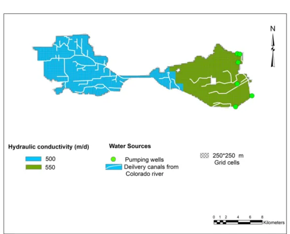
(6) 22. Kedir Mohammed Bushira·Jorge Ramírez Hernandez. Fig. 3. Distributions of calibrated horizontal hydraulic conductivity (Kh) for the 1st layer, water sources, and grids used for MF-FMP modeling.. characterize the hydrogeological units in the model area,. to meters for length and days for a time. The time frame of. data were reviewed on Transmissivity, specific storage and. the model simulation is 12 hydrologic years from 1st Octo-. storage coefficient from a previous parent MODFLOW. ber 1995 to 30th September 2006.. model study (Bushira. K. M, et al., 2017) and others (Feinstein et al., 2008; Rodriguez-Burgueño, 2012). The degree. 3.4. Landscape Attributes. of permeability in the first layer, in the horizontal directions. The assessment of sustainable yield and analysis of the. (Kh,) is spatially differentiated which contain two zones of. supply and demand components relative to the hydrologic. hydraulic conductivity (Fig. 3). The specific yield of Layer. cycle requires discretization of the irrigation unit 16 into. 1 was a constant value of 0.2. Vertical hydraulic conductiv-. subregions that can be used to estimate the water balance of. ity (Kv) in Layer 1 was 0.03 m/d. Layer 2 has an identical. land use and groundwater. In this study, the WBSs are. footprint to layer 1 and was designed to reflect a simplified. hydrologic entity delineated farm groups that are used to. state-of-knowledge of the model area geology. This layer. calculate the overall supply and demand components. represents the less hydrologically significant thick lower. through time. Irrigation unit 16 was grouped into 6 water. unit of consolidated to semiconsolidated mudstone- silt-. balance subregions (Fig. 4). These subregions represent a. stone and well-sorted sandstone of marine and continental. combination of virtual farms in the unit that can be used to. origin as described by other workers in the area. Layer 2. assess the inflow and outflow components of the hydro-. was designated a uniform (Kh) of 0.001 m/d and specific. logic cycle. This article presents the results of simulated. storage of 0.00003 1/m. Vertical hydraulic conductivity in. supply-constrained and demand-driven components across. layer 2 was assigned a value of 0.03 m/d.. the landscape for WBS1 on the eastern side and WBS3 on. Throughout the model, the units of measurements are set J. Soil Groundwater Environ. Vol. 24(5), p. 17~30, 2019. the western side (Fig. 4)..

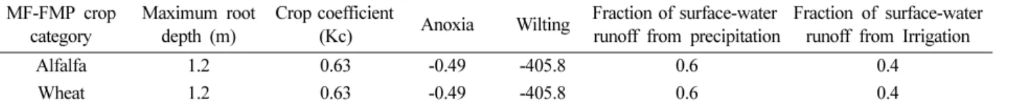
(7) MODFLOW-Farm Process Modeling for Determining Effects of Agricultural Activities on Groundwater Levels and Groundwater Recharge. 23. Fig. 4 (I) WBS and WBS id designation, (II) soil distribution and soil id designation, (III) boundary conditions and (IV) distributions of delivery canals for streamflow routing package (SFR).. The main types of crops grown in irrigation district 014. The irrigation efficiency for the study area was reviewed. are wheat (65%), alfalfa (19%), and cotton (8%). The main. from previous studies (Eliana, et al., 2012 and Feirstein. crops in the study area; irrigation unit 16 are wheat and. et al. 2008); an efficiency value of 0.65 to 0.85 is adopted in. alfalfa (Yamilett K.C. G 2009). The information used in the. this study.. study area regarding the main types of crop and their prop-. Four categories of soil are identified in the study area. erties for MF-FMP modeling were identified (Table 1 and. (Fig. 4). The spatial locations and distributions of crop. Table 2). These values are derived from the literature and. types, soil types and water balance subregions (farms) were. from related studies (Schmid and others, 2006a).. pre-prepared as an object shapefile in ArcGIS and exported J. Soil Groundwater Environ. Vol. 24(5), p. 17~30, 2019.

(8) 24. Kedir Mohammed Bushira·Jorge Ramírez Hernandez. Table 1. Summary of irrigation unit 16 virtual crop categories and properties MF-FMP crop category. Maximum root depth (m). Crop coefficient (Kc). Anoxia. Wilting. Alfalfa Wheat. 1.2 1.2. 0.63 0.63. -0.49 -0.49. -405.8 -405.8. Fraction of surface-water Fraction of surface-water runoff from precipitation runoff from Irrigation 0.6 0.6. 0.4 0.4. Table 2. Summary of fractions of transpiration and evaporation by year for irrigation unit 16 crop categories (virtual crops) MF-FMP Crop category. The fraction of transpiration (Ftr). The fraction of Evaporation from pre (Fep). The fraction of Evaporation from irrigation (Fei). Alfalfa Wheat. 0.05 0.05. 0.95 0.95. 0.1 0.1. to ModelMuse, a different soil, and farm id was assigned. the WEL package (Harbaugh and others, 2000) and the total. (Fig. 4). The drains of the irrigated agriculture were simu-. pumpage for each WBS (that is, virtual farm) is distributed. lated with the drain package in MODFLOW. The drain. among each of the farm wells within the WBS based on the. package for the study area was used and the drains set a. fraction of total pumping capacity (Schmid and others,. specified drain elevation that is about 1.8 m below the land. 2006a). A total of six groundwater wells are found in irri-. surface of drainage model cells (Fig. 4(III)) that are gener-. gation unit 16 which is located on the eastern edge on WBS. ally coincident with the regions identified as having drains.. 1 and WBS2.. The remaining border area was analyzed using general head boundary (GHB) (Fig. 4(III)).. The simulated temporal distribution of hydraulic head for the whole irrigation unit 16 was used to identify the effects of agricultural activities on groundwater level and the water. 3.5. Surface water and Groundwater Agricultural Supply. budget was used to detect groundwater recharge. In addition, the recharge to the aquifer was determined by analyz-. Surface-water inflows and outflows were simulated with. ing the water budget for each water balance subregions. a streamflow routing network composed of 55 stream seg-. (virtual farms). In this article, the landscape budgets for. ments representing the delivery canal which delivery sur-. WBS1 on the eastern side and WBS3 on the western side. face water from the Colorado River into the irrigation unit. are presented.. 16. This network (Fig. 4(IV)) was used to simulate the inflows and outflows along the major diversions. These fea-. 4. Results and Discussion. tures were simulated using the Streamflow-Routing Package (SFR2; Niswonger and Prudic, 2005); this head-. 4.1. Model calibration. dependent boundary condition allows for streamflow rout-. The trial and error basic head calibration was conducted. ing and the conveyance of overland runoff and the diver-. using the available observation points. Resulting values of. sion of water for irrigation.. the horizontal hydraulic conductivities for the first layer. Groundwater pumpage is a major component of the. after calibration are given in Fig. 3. The performance of the. hydrologic budget in Mexicali Valley and is used for agri-. calibration is illustrated by comparing simulated versus. cultural water supply. Irrigation district 014 which shares. observed groundwater heads. In view of the available head. the same aquifer with irrigation unit 16 includes more than. observation points, the result obtained is fairly acceptable,. 639 pumping wells used to supply water for irrigation. All. with an RME (root mean square error) of 0.02 m, a normal-. Farm wells are located in the first layer; simulated as a sin-. ized RMS of 2.1% and a correlation coefficient of 0.97.. gle-aquifer well (Schmid and others, 2006a) that collec-. Reported (measured) pumpage for the period 1995 through. tively supply water needed for irrigation for each WBS.. 2006 was available for WBS1 and WBS2. The totals of. Farm wells that are single-aquifer wells are simulated using. reported agricultural pumpage were compared with agricul-. J. Soil Groundwater Environ. Vol. 24(5), p. 17~30, 2019.

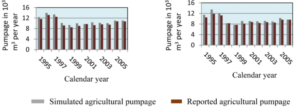
(9) MODFLOW-Farm Process Modeling for Determining Effects of Agricultural Activities on Groundwater Levels and Groundwater Recharge. 25. Fig. 5. Total annual reported and simulated agricultural pumpage for WBS1 (right) and WBS2 (left) for the period (1995-2006).. Table 3. Groundwater balance obtained from the MF-FMP model (whole irrigation unit 16) Inflow. Amount (104 m3). Storage Head dep bounds Stream leakage UZF recharge Farm net recharge.. 4.15 1.08 2.10 178.62 97.84. Outflow. Amount (104 m3). Storage 123.25 Drains 2.52 Head dep bounds 0.14 GW ET 123.16 Surface leakage 36.36 Farm wells 0.25 Inflow-Outflow -2.02*104 Percent discrepancy 0.71% Note: The net recharge is defined as inefficient losses to groundwater recharge after consumption due to excess irrigation and excess precipitation, reduced by losses to surface-water runoff and ET from groundwater (Schmid and others, 2006a).. tural pumpage estimated through the simulation of water. The resulting groundwater balance is given in Table 3.. consumption by the Farm Process used in the study area.. The source of water to the groundwater reservoirs in the. The reported agricultural pumpage located at WBS1 and. study area is through agricultural recharge, which amounts. WBS2 were used as additional calibration targets.. in total to 97.84*104 m3. Leakage from the stream which. Simulated and reported total agricultural pumpage are. amounts 2.10*104 m3 and lateral inflows which amount. compared for the 2 WBSs (Fig. 5). The model slightly over-. 1.08*104 m3 are other components of inflows. About 2.52. estimates agricultural pumpage. The percentages of total. *104 m3 of groundwater drains out of the system. The study. reported and simulated agricultural pumpage by WBS are. area experiences high groundwater evaporation amount. also comparable, within a few percent, for the two subre-. about 123.16*104 m3. The model balance error is very small,. gions. The annual total and total agricultural pumpage (Fig.. i.e. -0.71%, which shows that the model has converged. 5) are comparable between reported and simulated values. accurately. The discrepancy is negative; indicating that out-. for these 12 years. For the WBS1 and WBS2 model, the. going groundwater from the study area is higher than. average annual differences (reported minus simulated) for. incoming groundwater (recharge) which shows aquifer. total agricultural were -671 m3/yr. and -570 m3/yr. for the. drawdown.. period 1995–2006, respectively. This represents average differences of about -0.54 and -0.49 percent of the reported. 5. Discussion. agricultural pumpage, respectively. These results show that the simulated pumpage is within the range of uncertainty of the reported pumpage.. As indicated by the simulated potentiometric level (Fig. 6), groundwater flows laterally from the highest elevation J. Soil Groundwater Environ. Vol. 24(5), p. 17~30, 2019.

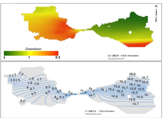
(10) 26. Kedir Mohammed Bushira·Jorge Ramírez Hernandez. Fig. 6. (I) Simulated drawdown (m) and (II) simulated hydraulic heads (m a.s.l.) for irrigation unit 16.. Fig. 7. Farm delivery components and the inflows and outflows for two water-balance subregions (WBS1, top, and WBS3, bottom) from 1995 to 2006. Recharge and runoff, refer the second axis.. points to the lowlands toward the Gulf of California. Simu-. shows a drawdown ranges from 3 m to 0.3 m. The draw-. lated water levels range from 19.6 m in the highland areas. down is higher in the northeastern modeling area which is. to less than 10 m in the lowland. The three-dimensional. expected because most of the groundwater pumping wells. modeling of groundwater in the study area shows aquifer. existed nearby.. drawdown for the study period. The drawdown map (Fig. 6) J. Soil Groundwater Environ. Vol. 24(5), p. 17~30, 2019. Figure 7 shows the simulated total farm delivery require-.

(11) MODFLOW-Farm Process Modeling for Determining Effects of Agricultural Activities on Groundwater Levels and Groundwater Recharge. 27. Fig. 8. Graph showing the percentages of total Landscape (LS) inflows and outflows for two water-balance areas from 1995 to 2006 as part of conjunctive use simulated by MF-FMP Note: water budgets are relative to farm units; direct evaporation and transpiration of groundwater uptake on both the inflow and outflows because those fluxes are passing through the land surface (from groundwater to atmosphere/plants through the land surface). Refer section” MF-FMP Features” in this article or referred to Schmid et al. (2006a) for more detail.. ment for irrigation for a WBS1 and WBS3 for the 12- year. regions (Fig. 7, yellow color).. period from 1995 to 2006 and Figure 8 summarizes the. The simulated component for WBS 1 and WBS 3 (Fig. 7). overall 12-year WBS landscape hydrologic budgets for. show that groundwater recharge is derived from agricul-. WBS1 and WBS3.. tural supplies nothing that the precipitation is lost due to. The results show that WBS1, which constitutes the eastern part of the modeling area, receives comparably more. evapotranspiration. Fig. 7 also demonstrates a reducing trend recharge.. runoff and after the year 1999, lesser recharge than WBS3,. Groundwater-level decline and related storage depletion. which constitutes the western part of the modeling area.. are occurring in this area as evapotranspiration (ET) from. The simulated total farm delivery requirement (TFDR). groundwater uptake are about 3% and 4% (Fig. 8, inflow). shows that TFDR for WBS1 is fulfilled by 73% from the. and recharge to the groundwater is about 19% and 21% on. diversion of the Colorado River through delivery canals and. the landscape (Fig. 8, outflow) for WBS1 and WBS 3. 27% from groundwater pumping. In contrast, the TFDR of. respectively. Evapotranspiration from groundwater, water. WBS3 mainly depends on the diversion of the Colorado. from agriculture wells and routed surface water deliveries. River. There is a significant component of evapotranspira-. supplement the crop consumptive use for WBS1 and the. tion (ET) derived from irrigation in both water balance sub-. crop consumptive use of WBS 3 is supplemented by surJ. Soil Groundwater Environ. Vol. 24(5), p. 17~30, 2019.

(12) 28. Kedir Mohammed Bushira·Jorge Ramírez Hernandez. face water deliveries and evapotranspiration from ground-. 123.16*104 m3. The average negative change in storage. water (Fig. 8).. is indicating that outgoing groundwater from the study. For each WBS represented by many model cells, the results shown in Figures 6 to 7 are the aggregate of the cells. area is higher than incoming groundwater (recharge) which shows aquifer depletion.. involved. Crop types, crop coefficients, potential or speci-. • Calibration of the model using the available observa-. fied evapotranspiration, and other characteristics are defined. tions of groundwater levels gives a relatively good fit. for each cell, and results such as crop irrigation require-. with an RMS of 0.02 m and a normalized RMS of 2.1%. ments are simulated for each cell.. with a correlation coefficient of 0.97. The reported agri-. Integrated hydrologic models are essential in the analysis. cultural pumpage located at WBS1 and WBS2 was used. of conjunctive use issues; if not, it might be difficult to ana-. as an additional calibration target that, the simulated. lyze the flows and interactions between the head and flow-. pumpage is within the range of uncertainty of the reported. dependent components. MF-FMP is one of the integrated. pumpage. The average annual differences (reported. hydrologic models able to simulate coupled processes across. minus simulated) for total agricultural were -671 m3/yr.. the landscape, surface water and groundwater components. and -570 m3/yr. Which represents average differences of. of the hydrologic cycle.. about -0.54 and -0.49 percent of the reported agricul-. This study shows how WBS can be used to organize. tural pumpage for WBS1 and WBS2 respectively.. input data and simulated results. Farm process (FMP) input. • The simulated potentiometric level shows a hydraulic. files was easily constructed, updated, and maintained using. head range from 19.6 m in some areas to less than 10 m. soil, well, and crop data that did not require substantial. in the lowlands. Groundwater flows toward the Gulf of. external estimation of inflows and outflows (pumpage,. California.. recharge, evapotranspiration, runoff, surface water deliver-. • The simulated MF-FMP inflow-outflow analysis shows. ies, etc.) prior to simulation. Because these hydrologic com-. that the WBS1, which constitutes the eastern part of the. ponents are simulated separately, the flows and movement. modeling area, receives comparably more runoff and. were easily analyzed.. after the year 1999, lesser recharge than WBS3, which constitutes the western part of the modeling area.. 6. Conclusions. • The simulated component for WBS 1 and WBS 3 confirmed that groundwater recharge is derived from agri-. The sustainability of water resources in part depends on the ability to monitor our aquifers and to simulate and ana-. cultural supplies nothing that the precipitation is lost due to evapotranspiration.. lyze all the components of complex hydrologic systems,. • The landscape budget for WBS1 and WBS 3 shows. including groundwater, surface water, and landscape com-. evapotranspiration (ET) from groundwater uptake are. ponents. A regional groundwater flow model on irrigation. about 3% and 4% and recharge to the groundwater is. unit 16 was developed and calibrated against available. about 19% and 21% respectively.. groundwater level observations and measured agricultural. • The modeling effort on irrigation unit 16 shows that the. pumpage, which converges to a solution with a small water. aquifer was drawn downed up to 3 m in some areas and. balance error. A conceptual model of the study area with. drawdown was higher in the northeastern region than. two layers is defined to identify the effects of agricultural activities on groundwater level and groundwater recharges. The main conclusions drawn from the model are:. western regions. • The MF-FMP modeling on selected WBS showed that recharge to the aquifer occurring in response to irriga-. • The source of water to the groundwater reservoirs in the. tion supplies because there is little precipitation exists;. study area is through net-agricultural recharge, which. which eventually lost before reaching to the aquifer.. amounts in total to 97.84*104 m3. The study area expe-. Routed surface water delivery, pumping delivery for. rienced high groundwater evaporation amount about. irrigation and evaporation from groundwater uptakes are. J. Soil Groundwater Environ. Vol. 24(5), p. 17~30, 2019.

(13) MODFLOW-Farm Process Modeling for Determining Effects of Agricultural Activities on Groundwater Levels and Groundwater Recharge. 29. the main landscape inflow components for eastern areas. River Delta, Mexico. Tesis de Maestría. Tucson, AZ.. (WBS1) in addition to precipitation. Crop consumptive. Gastil, R.G., Krummenacher, D., and Minch, J.A., 1979, The record of Cenozoic volcanism around the Gulf of California, Geological Society of America Bulletin, 90, 839-857.. use in the western side (WBS3) is supplemented by the routed surface water delivery, evaporation from groundwater and precipitation. The authors believe that these results are very important for future conjunctive water resources management in the region and this work is the first and unique example in the region which might be a guide for development of the integrated hydrologic model using MF-FMP for whole irrigation district 014 which is in need and other agricultural regions which seek integrated modeling with a similar geological environment. Monitoring of diversion rates from the Colorado River to each farm on a better scale as a function of time and detail database on agricultural crops are recommended for future model development.. Acknowledgment The authors would like to acknowledge Autonomous University of Baja California (UABC), Agencia Mexicana de Cooperación Internacional para el Desarrollo de la Secretaria de Relaciones Exteriores del Gobierno Mexicano, and Arba Minch University for all type of support they provided.. References Barragan, R. M., P. Birkle, E. Portugal M., V. M. Arellano G., and J. Alvarez R., 2001, Geochemical survey of medium temperature geothermal resources from the Baja California peninsula and Sonora, Mexico, Journal of Volcanology and Geothermal Research, 110, 101-119, PII: S0377-0273(01)00205-0. Bushira, K.M., Ramirez-Hernández, J., and Zhuping, S., 2017, Surface and groundwater flow modeling for calibrating steady state using MODFLOW in Colorado River Delta, Baja California, Mexico, Journal of Modeling earth systems and Environment.no. 3, 815-824.. Harshbarger, J.W., 1971, Overview report of hydrology and water development, Colorado Delta, United States and Mexico, Preliminary Report PR-235-77-2, Prepared for International Boundary and Water Commission United States Section, Tucson AZ, USA. Harbaugh, A.W., Banta, E.R., Hill, M.C., and McDonald, M.G., 2000, MODFLOW-2000, U.S. Geological Survey modular ground-water model-User guide to modularization concepts and the ground-water flow process: U.S. Geological Survey OpenFile Report 2000-92, 121 p., http://pubs.er.usgs.gov/publication/ ofr200092. Harbaugh, A.W., 2005. MODFLOW-2005: the U.S. Geological Survey modular ground-water model-the ground-water flow process: U.S. Geological Survey Techniques and Methods 6A16, variously paginated, http://pubs.er.usgs.gov/publication/ tm6A16. Hillel, D. (2008) Soil chemical attributes and processes, Soil in the environment: crucible of terrestrial life, Chapt 10. Academic Press, San Diego, pp. 135-150. Hill, B.M., 1993, Hydrogeology, numerical model and scenario simulations of the Yuma area groundwater flow model Arizona, California, and Mexico, Modeling Report no. 7, Arizona Department of Water Resources, Phoenix AZ, USA. Mock, P.A., Burnett, E.E., and Hammett, B.A., 1988, Digital computer model study of Yuma area groundwater problems associated with increased river flows in the lower Colorado River from January 1983 to June 1984, Arizona Department of Water Resources Open-File Report No. 6, Phoenix AZ, USA. Niswonger, R.G., Prudic, D.E., and Regan, R.S., 2006. Documentation of the Unsaturated-Zone Flow (UZF1) Package for modeling unsaturated flow between the land surface and the water table with MODFLOW-2005. U.S. Geological Survey Techniques and Methods 6-A19. Niswonger, R.G. and Prudic, D.E., 2005, Documentation of the streamflow-routing (SFR2) package to include unsaturated flow beneath streams-A modification to SFR1: U.S. Geological Survey Techniques and Methods 6-A13, 51 p., http://pubs.er.usgs. gov/publication/tm6A13.. Chavez, R.E., Lazaro-Mancilla, O., Campos-Enriquez, J.O., and Flores-Marquez, E.L., 1999, Basement topography of the Mexicali Valley from spectral and ideal body analysis of gravity data, Journal of South American Earth Sciences, 12, 579-587, PII: S0895-9811(99)00041-3.. Olmsted, F., Loeltz, O.y., and Irelan, B., 1973, Geohydrology of the Yuma Area, Arizona, and California, Geological Survey Professional Paper 486-H, United States Government Printing Office Washington, DC.. Feirstein, E., Zamora-Arroyo, F., Vionnet, L.y., Maddock, T. 2008, Simulation of groundwater conditions in the Colorado. Pacheco, M., Martin-Barajas, A., Elders, W., Espinosa-Cardena, J.M., Helenes, J., and Segura, A., 2006, Stratigraphy and strucJ. Soil Groundwater Environ. Vol. 24(5), p. 17~30, 2019.

(14) 30. Kedir Mohammed Bushira·Jorge Ramírez Hernandez. ture of the Altar basin of NW Sonora: implications for the history of the Colorado River Delta and the Salton trough, Revista Mexicana de Ciencias Geologicas, 23(1), 1-22.. Baja California Sur, Mexico, in Frizzell, V.A., Jr., Geology of the Baja California Peninsula, Society of Economic Paleontologists and Mineralogists, 39, 239-251.. Portugal, E., Izquierdo, G., Truesdell, A., and Alvarez, J., 2005, The geochemistry and isotope hydrology of the Southern Mexicali Valley in the area of the Cerro Prieto, Baja California (Mexico) geothermal field, Journal of Hydrology, 313, 132-148.. Schmid, W. and Hanson, R.T., 2009b. The Farm Process Version 2 (FMP2) for MODFLOW-2005 – Modifications and Upgrades to FMP1. U.S. Geological Survey Techniques in Water Resources Investigations, Book 6, Ch. A32.. Puente, I.C. and A. De La Pena L., 1979, Geology of the Cerro Prieto geothermal field, Geothermics, 8, 155-175.. Schmid, W., 2004, A Farm Package for MODFLOW-2000: Simulation of Irrigation Demand and Conjunctively Managed Surface-Water and Ground-Water Supply. Ph.D. Dissertation. Department of Hydrology and Water Resources, the University of Arizona.. Richard B. Winston. 2009, ModelMuse-A Graphical User Interface for MODFLOW-2005 and PHAST. Roman-Calleros, J. and Ramírez-Hernández, J., 2003. Interdependent Border Water Supply Issues: The Imperial and Mexicali Valleys. In: Michel S. (Eds.), The U.S.-Mexican border environment: Binational water management planning, San Diego State University Press, San Diego, California, Chap: 2, pp. 95144. Rodríguez-Burgueño, J., 2012, Modelación geohidrológica transitoria de la relación acuífero-río de la zona FFCC -vado Carranza del río Colorado con propósito de manejo de la zona riparia., Master Eng., Universidad Autónoma de Baja California, Mexicali, B.C.. Schmid, W., Hanson, R.T., Maddock III, T.M., and Leake, S.A., 2006a. User’s guide for the Farm Package (FMP1) for the U.S. Geological Survey’s modular three-dimensional finite-difference groundwater flow model, MODFLOW- 2000. U.S. Geological Survey Techniques and Scientific Methods Report Book 6, Chapter A17. Schmid, W., Hanson, R.T., and Maddock III, T.M., 2006b, Overview and Advances in the Farm Process for MODFLOW2000. MODFLOW and MORE 2006. Managing Groundwater Systems-Conference Proceedings, 23-27.. Schmid, W. and Hanson, R.T., 2009a, Appendix 1, Supplemental Information-Modifications to Modflow-2000 Packages and Processes. In Ground-Water Availability of California’s Central Valley., ed. C.C. Faunt, 213-225. U.S. Geological Survey Professional Paper 1766.. Smith, J.T., 1984, Miocene and Pliocene mar~ne mollusks and preliminary correlations, Viscaino Peninsula to Arroyo La Purisima, northwestern Baja California Sur, Mexico, in Frizzell, V.A., Jr., Geology of the Baja California Peninsula: Society of Economic Paleontologists and Mineralogists, 39, 197-217.. Sawlan, M.G. and Smith, J.G., 1984, Petrologic characteristics, age, and tectonic setting of Neogene volcanic rocks in northern. Sykes, G.G., 1935, The Colorado Delta, Carnegie Institution of Washington, Washington DC, USA.. J. Soil Groundwater Environ. Vol. 24(5), p. 17~30, 2019.

(15)