A Study on Imputation using Adjusted Cohen A Study on Imputation using Adjusted Cohen A Study on Imputation using Adjusted Cohen A Study on Imputation using Adjusted Cohen
Method MethodMethod Method1)1)1)1)
Sung-Suk Chung Sung-Suk ChungSung-Suk Chung
Sung-Suk Chung2)2)2)2) ․․․․ Young-Min ChunYoung-Min ChunYoung-Min ChunYoung-Min Chun3)3)3)3) ․․․․ Sun-Kyung LeeSun-Kyung LeeSun-Kyung LeeSun-Kyung Lee4)4)4)4)
Abstract Abstract Abstract Abstract
Many studies have been done to develop procedures to deal with missing values. Most common method is to reassign the other values to the missing data. The purpose of our study is to suggest adjusted Cohen methods and to compare the efficiency of them with other methods through a simulation study. The adjusted Cohen methods use an auxiliary variable to arrange ranking of the variable with missing values. It leads to a reduced mean square error(MSE) compared with the Cohen method.
Keywords Keywords Keywords
Keywords : Adjusted Cohen method, Imputation method, Missing data patterns, Missing mechanisms
1. Introduction 1. Introduction1. Introduction 1. Introduction
Most statistical analyses are performed by complete data but missing values almost always exist in real data. Missing data may occur due to different reasons such as death of patients, equipment malfunctions, refusal of respondents to answer certain questions, and so on. If we don't include all the observations with missing values, the loss of information might be significant. This approach also ignores the possible systematic difference between the complete cases and incomplete cases, and the resulting inference may not be appropriate, especially
1) This work was supported by grant No. R01-2005-000-10752-0 from Ministry of Science and Technology(Korea Science and Engineering Foundation).
2) Professor, Div. of Mathematics and Statistical Informatics (Institute of Applied Statistics), Chonbuk National University, Jeonju, Korea
E-mail : [email protected]
3) Doctoral Course, Dept. of Computer and Statistical Informatics, Chonbuk National University, Jeonju, Korea
E-mail : [email protected]
4) Master, Dept. of Statistical Informatics, Chonbuk National University, Jeonju, Korea E-mail : [email protected]
when the missing rate of data is high. Therefore many studies have been done to develop procedures to deal with missing values.
There are two types of nonresponse: unit nonresponse, in which the entire observation unit is missing, and item nonresponse, in which more than one item is missing for an observation unit. One of the most common methods to deal with unit nonresponse is weighting adjustment which is to reassign the weights of the nonresponse to the response. Common methods for item nonresponse are imputation methods. Imputation is a general and flexible method for handling missing data problems. Imputation is a procedure that replaces the missing values in a data set by predicted or simulated values. The basic object of imputation is to allow end users to apply their existing analysis tools to any dataset with missing values using the same command structure and output standards as if there were no missing data.
Imputation methods are divided into single imputation and multiple imputation.
Single imputation substitutes a value for each missing value, so it is easy to use and simple, but it has serious drawbacks like reduction variance. Multiple imputation replaces each missing value with more than one value to represent imputation uncertainty. It offers valid result but it is a burden to impute missing values and analysis for several times.
The purpose of this study is to suggest adjusted Cohen methods and to compare the efficiency of them with other methods through a simulation study.
The adjusted Cohen methods use an auxiliary variable to arrange ranking of the variable with missing values. It leads to a reduced mean square error(MSE) compared with the Cohen method. Cohen(1996) proposed a new approach that complements the underestimation variance of mean imputation, but it tends to inflate the MSE. We are not concerned here with categorical variables involving missing values.
This study consists of five sections. Section 1 reviews the missing data problems. Section 2 explains missing data mechanisms and patterns. Missing data mechanisms are MCAR, MAR and NMAR and missing data patterns are monotone and arbitrary. Section 3 discusses several imputation methods that are mean imputation, cohen method, regression imputation, and multiple imputation.
Section 4 suggests the adjusted Cohen methods and reports the results of a simulation study. Section 5 comments about conclusions and future directions.
2. Missing Mechanisms and Patterns 2. Missing Mechanisms and Patterns 2. Missing Mechanisms and Patterns 2. Missing Mechanisms and Patterns 2.1 Missing Mechanisms
2.1 Missing Mechanisms 2.1 Missing Mechanisms 2.1 Missing Mechanisms
Missing mechanisms concern the relationship between missingness and the values of variables in the data matrix. These are MCAR, MAR and NMAR(Little and Rubin(2002)).
The missing data for a variable Y is "Missing Completely at Random(MCAR)", if the probability of having a missing value for Y is unrelated to the value of Y itself or any other variable in the data set.
For example, income is MCAR, if two conditions are satisfied. One is that people who do not report their income have, on the average, the same income as people who do report income. The other is that each of the other variables in the data set would have to be the same, on average, for the people who did not report their income and the people who did report their income. MCAR is the best situation to treat the missing data.
The missing data for a variable Y is "Missing At Random(MAR)", if the probability of the missing data of Y is unrelated to the value of Y, but to other variables. MCAR is a special type of MAR and MAR is much weaker assumption than MCAR.
For example, income is MAR, if the probability of missing data of income depends on martial status, but within each category of martial status, the probability of missing data on income is unrelated to the value of income. MAR and MCAR are ignorable missingness.
The missing data for a variable Y is "Not Missing at Random(NMAR)", if the probability of missing data of Y is related to the actual value of the missing data.
For example, if high income households are less likely to report their income even after adjusting for other variables, then the probability of missing income is not ignorable. This is the most difficult condition to modeling.
2.2 Missing Data Patterns 2.2 Missing Data Patterns 2.2 Missing Data Patterns 2.2 Missing Data Patterns
Missing data patterns describe which values are observed in the data matrix and which are missing(Little and Rubin(2002)). A data set is said to have monotone missing patterns when the missing particular variable implies that all subsequent variables are all missing, for . Simpler imputation methods can be used, if the missing data patterns are monotone, however a monotone pattern is uncommon in most real data.
In an arbitrary pattern, missing data can occur anywhere. The MCMC algorithm, introduced in section 3.4.1, is appropriate for missing data which has an
arbitrary pattern. Another way to handle a missing data set with an arbitrary pattern is to use the MCMC algorithm to impute enough values to make the missing data patterns monotone. Then, a simpler imputation method can be used.
3. Imputation Methods 3. Imputation Methods 3. Imputation Methods 3. Imputation Methods 3.1 Mean Imputation
3.1 Mean Imputation 3.1 Mean Imputation 3.1 Mean Imputation
Mean imputation is the simplest and the oldest method. This method replaces missing values with the mean of observed values. The mean is formed in conditional or unconditional situation.
The mean of the observed values is given as
. With
unconditional mean imputation, the mean estimator is given as
and the variance estimator is given as
. The notation is random variable, is sample size, is a number of observed values of .
Under MCAR assumption, is unbiased but biased in general and the variance estimator underestimates the variance by a factor of
. The covariance is also underestimated by this method and if the variables are highly correlated, this method cannot be recommended.
Conditional mean imputation first uses some auxiliary variables to form adjustment classes, and then replaces missing values in each class with its sample mean.
3.2 Cohen Method 3.2 Cohen Method 3.2 Cohen Method 3.2 Cohen Method
Cohen(1996) suggested an approach that makes use of imputed values distributed more diffusely than the observed data. For example, instead of imputing the mean for all the missing values, half of the missing values are imputed by
and the other half by
, where . This
approach is effective to adjust reduced variance of mean imputation.
3.3 Regression Imputation 3.3 Regression Imputation 3.3 Regression Imputation 3.3 Regression Imputation
The idea of this method is that missing values are replaced by predicted values derived from a regression model. In regression imputation, missing values of a variable are imputed by predicted values from the regression of on
⋯ ⋯ , based on the complete cases, where
⋯ ⋯ are fully observed and is observed for the
observations. The result equation is given as
⋯ ⋯ .
This method requires a model and assumes that missing data are MAR. The drawback of regression imputation is that this inflates correlations and becomes difficult in multivariate data when more than one variable has missing values, i.e.
a data set that has multiple missing.
The stochastic regression imputation method replaces a missing value by a value predicted by regression imputation plus a random error. The form of the equation is like where is a random value from a normal distribution with zero mean and the variance equal to the residual variance in the regression.
3.4 Multiple Imputation 3.4 Multiple Imputation 3.4 Multiple Imputation 3.4 Multiple Imputation
Multiple imputation is one of the most attractive methods for general purpose handling of missing data in multivariate analysis. It is first proposed by Rubin(1976) and elaborated in his(1987) book. Rubin described multiple imputation as a three-step process.
Step 1 : The missing data are imputed in m times to generate m complete
・
data sets.
Step 2 : The m complete data sets are analyzed by using standard statistical
・
analysis.
Step 3 : The results from the m complete data sets are combined to produce
・
one overall analysis.
Multiple imputation requires MAR or MCAR assumption and represents a random sample of the missing values rather than attempting to estimate each missing value.
This process results in valid statistical inferences that precisely reflect the uncertainty due to missing values. Uncertainty is accounted by creating different versions of the missing data and observing the variability between imputed data
sets. The disadvantage of multiple imputation is that it takes more work to create the imputations and analyze the results than single imputation and the statistical principles behind multiple imputation are not trivial.
3.4.1 Imputation step using Markov Chain Monte Carlo(MCMC) 3.4.1 Imputation step using Markov Chain Monte Carlo(MCMC) 3.4.1 Imputation step using Markov Chain Monte Carlo(MCMC) 3.4.1 Imputation step using Markov Chain Monte Carlo(MCMC)
In the imputation step, a variety of imputation methods have been used. The method of choice relies upon the type of missing data patterns. For an monotone missing data pattern, simple methods have been proposed. Propensity methods or predictive mean matching is appropriate for continuous variables and discriminant analysis or logistic regression for discrete variables. For an arbitrary missing data pattern, the Markov Chain Monte Carlo(MCMC) that assumes multivariate normal distribution has been suggested.
A Markov chain is a sequence of random variables in which the distribution of each element depends on the value of the previous one.
The first step computes mean vector and covariance matrix from the data that does not have missing values to estimate the prior distribution. Next, the imputation step simulates values for missing values by randomly selecting a value from the available distribution of values. The posterior steps recomputes mean vector and covariance matrix with the imputed values from the imputation step.
This is posterior distribution. Imputation step and posterior step are iterated until mean vector and covariance matrix are unchanging as we iterate.
When we denote the variables with missing values for observation i by
and the variables with observed values by , the imputation step draws from with a current parameter estimate at
iteration. The posterior step draws from . This creates a Markov chain ⋯ ⋯, which converges in distribution to .
3.4.2 Combination results 3.4.2 Combination results 3.4.2 Combination results 3.4.2 Combination results
Combining inference from the imputed data sets is done using rules conformed by Rubin(1987). Rubin detailed that combining the estimates of the point and variance for a parameter of interest. When and are the point and variance estimates from the th imputed data set, , the point estimate for from multiple imputation is the average of the complete data estimates :
.
The total variance is expressed by the formula
, where
, . is the "within imputation variance"
and B is the "between imputation variance". The former means the natural variability and the latter estimates uncertainty caused by missing data.
3.4.3 Multiple imputation efficiency 3.4.3 Multiple imputation efficiency 3.4.3 Multiple imputation efficiency 3.4.3 Multiple imputation efficiency
When we generate complete sets, we have to determine how many.
Then, we can consult the relative efficiency of an estimate based on imputation which is showed by Rubin(1987,p.114). The relative efficiency(RE) is approximately given as a function of and . , where
,
. The ratio is called the relative increase in variance due to nonresponse and is the rate of missing information for the quantity being estimated(Rubin, 1987). The following Table 1 shows the RE with different value of and . Surprisingly, for cases with little missing information, only 3 10 imputations are enough.~
m .1 .2 .3 .5 .7
3 0.9677 0.9375 0.9091 0.8571 0.8108 5 0.9804 0.9615 0.9434 0.9091 0.8772 10 0.9901 0.9804 0.9709 0.9524 0.9346 20 0.9950 0.9901 0.9852 0.9756 0.9662
<Table 1> Relative efficiency
Besides there are hot deck imputation, cold deck imputation, ratio imputation, and EM algorithm, etc. With hot deck imputation, missing values are replaced by values from the responding units in the sample that are derived sequentially, hierarchically or via a distance function. In the cold deck method, missing values are replaced by values from an external source, such as a value from a previous result of the same survey. In ratio imputation,
is used as imputed values for the -th missing value. This ratio imputation may provide very precise imputation if the missingness of mainly depends on a highly correlated an auxiliary variable . The EM algorithm is a very general
iterative algorithm for maximum likelihood estimation in an incomplete data problem(Little and Rubin(1987)). This method replaces the missing values by using observed values and a parameter and then reestimates the parameter based on observed values and the imputed values until iterating converges.
4. Adjusted Cohen Methods and a Simulation Study 4. Adjusted Cohen Methods and a Simulation Study 4. Adjusted Cohen Methods and a Simulation Study 4. Adjusted Cohen Methods and a Simulation Study 4.1 Adjusted Cohen Methods
4.1 Adjusted Cohen Methods 4.1 Adjusted Cohen Methods 4.1 Adjusted Cohen Methods
We reviewed the imputation methods. According to Scheffer(2002), multiple imputation is always better than case deletion or single imputation. Also many statistical software packages support multiple imputation. However, Horton and Lipsitz(2001) mentioned that none of the packages are clearly superior and they remain in large part of a complicated black box whose output can be difficult to interpret it in their study. This ultimately makes end users shun its use.
Therefore, this study proposes a new approach that improves drawback of single imputation. The Cohen method was introduced in 3.2. This approach complements the underestimation of variance that is the chief drawback of mean imputation.
However, this method has a result even worse than mean imputation when comparing mean square error(MSE). It leads to inflation of MSE. Moreover, it tends to overestimate variance under MCAR assumption and it is not effective to adjust estimates of means.
This study suggests adjusted Cohen methods. This approach uses an auxiliary variable to arrange ranking of the variable with missing values, under the assumption that the auxiliary variable is fully observed. The missing values are imputed by more diversified values after sorting the variable with missing values by an auxiliary variable. Following figures show adjusted Cohen methods.
The first, two values can be used to impute like Cohen method. This method is diagrammed as figure 1. In the adjusted Cohen method 1, if a missing value is within the first 50% of ranking, the missing value is imputed by
.The second, mean of observed values can be added. This makes the adjusted Cohen method 2. The adjusted Cohen method 3 and 4 use four different values to impute, but percentage of ranking is unlike. The adjusted Cohen method 5 and 6 use five different values involving the mean of the observed values to impute, but also percentage of ranking is unlike. However, we have to conform that the variable with missing values has positive correlation with the auxiliary variable; if negative correlation exists, we can convert a sign between and
or
.The adjusted Cohen methods lower MSE and are useful to complement overestimation of variance under MCAR assumption. Mean estimates of the adjusted Cohen methods are mediated under MAR and NMAR, while the Cohen method has the same mean estimate with mean imputation. These methods don't need a model like regression imputation, and can also be used in multiple missing unless there is no variable to use as an auxiliary variable.
In the next section, a simulation study is performed to compare the efficiency of each adjusted Cohen method and with other imputation methods.
50%
50% obs
obs obs obs
j D
n n y n
1 1
)
( −
−
− +
obs obs
obs obs
j D
n n y n
1 1
)
( −
−
+ +
50%
50% obs
obs obs obs
j D
n n y n
1 1
)
( −
−
− +
obs obs
obs obs
j D
n n y n
1 1
)
( −
−
+ +
<Figure 1>
Adjusted Cohen method 1
35%
30%
35%
obs obs
obs obs
j D
n n y n
1 1
)
( −
−
− +
obs obs
obs obs
j D
n n y n
1 1
)
( −
− + +
) (obs
yj
35%
30%
35%
obs obs
obs obs
j D
n n y n
1 1
)
( −
−
− +
obs obs
obs obs
j D
n n y n
1 1
)
( −
− + +
) (obs
yj
<Figure 2>
Adjusted Cohen method 2
25%
25%
25%
25%
obs obs
obs obs
j D
n n y n
1 1
)
( −
−
− +
obs obs
obs obs
j D
n n y n
1 1 2
1
)
( −
−
− +
obs obs
obs obs
j D
n n y n
1 1 2
1
)
( −
− + +
obs obs
obs obs
j D
n n y n
1 1
)
( −
− + +
25%
25%
25%
25%
obs obs
obs obs
j D
n n y n
1 1
)
( −
−
− +
obs obs
obs obs
j D
n n y n
1 1 2
1
)
( −
−
− +
obs obs
obs obs
j D
n n y n
1 1 2
1
)
( −
− + +
obs obs
obs obs
j D
n n y n
1 1
)
( −
− + +
<Figure 3>
Adjusted Cohen method 3
20%
30%
30%
20%
obs obs
obs obs
j D
n n y n
1 1
)
( −
− + +
obs obs
obs obs
j D
n n y n
1 1
)
( −
−
− +
obs obs
obs obs
j D
n n y n
1 1 2
1
)
( −
−
− +
obs obs
obs obs
j D
n n y n
1 1 2
1
)
( −
− + +
20%
30%
30%
20%
obs obs
obs obs
j D
n n y n
1 1
)
( −
− + +
obs obs
obs obs
j D
n n y n
1 1
)
( −
−
− +
obs obs
obs obs
j D
n n y n
1 1 2
1
)
( −
−
− +
obs obs
obs obs
j D
n n y n
1 1 2
1
)
( −
− + +
<Figure 4>
Adjusted Cohen method 4
20%
20%
20%
20%
20%
obs obs
obs obs
j D
n n y n
1 1
)
( −
− + +
obs obs
obs obs
j D
n n y n
1 1 2
1
)
( −
− + +
obs obs
obs obs
j D
n n y n
1 1 2
1
)
( −
−
− +
obs obs
obs obs
j D
n n y n
1 1
)
( −
−
− +
) (obs
yj
20%
20%
20%
20%
20%
obs obs
obs obs
j D
n n y n
1 1
)
( −
− + +
obs obs
obs obs
j D
n n y n
1 1 2
1
)
( −
− + +
obs obs
obs obs
j D
n n y n
1 1 2
1
)
( −
−
− +
obs obs
obs obs
j D
n n y n
1 1
)
( −
−
− +
) (obs
yj
<Figure 5>
Adjusted Cohen method 5
10%
30%
20%
30%
10%
obs obs
obs obs
j D
n n y n
1 1
)
( −
− + +
obs obs
obs obs
j D
n n y n
1 1 2
1
)
( −
− + +
obs obs
obs obs
j D
n n y n
1 1 2
1
)
( −
−
− +
obs obs
obs obs
j D
n n y n
1 1
)
( −
−
− +
) (obs
yj
10%
30%
20%
30%
10%
obs obs
obs obs
j D
n n y n
1 1
)
( −
− + +
obs obs
obs obs
j D
n n y n
1 1 2
1
)
( −
− + +
obs obs
obs obs
j D
n n y n
1 1 2
1
)
( −
−
− +
obs obs
obs obs
j D
n n y n
1 1
)
( −
−
− +
) (obs
yj
<Figure 6>
Adjusted Cohen method 6
4.2 A Simulation Study 4.2 A Simulation Study 4.2 A Simulation Study 4.2 A Simulation Study
4.2.1 Simulation design 4.2.1 Simulation design 4.2.1 Simulation design 4.2.1 Simulation design (1) Data
Simulation is performed by Iris data and generated data. Table 2 shows detailed information.
data number of unit variables
Iris 150 (50 units of each of 3 species )
sepal length(SL)
・ ・ sepal width(SW)
petal length(PL)
・ ・ petal width(PW)
species of iris (categorical variable)
・
Generated 1000 ・ ∼ ・ ∼ ・ ∼
・ , where ∼
<Table 2> Simulation design of data
(2) Missing mechanisms
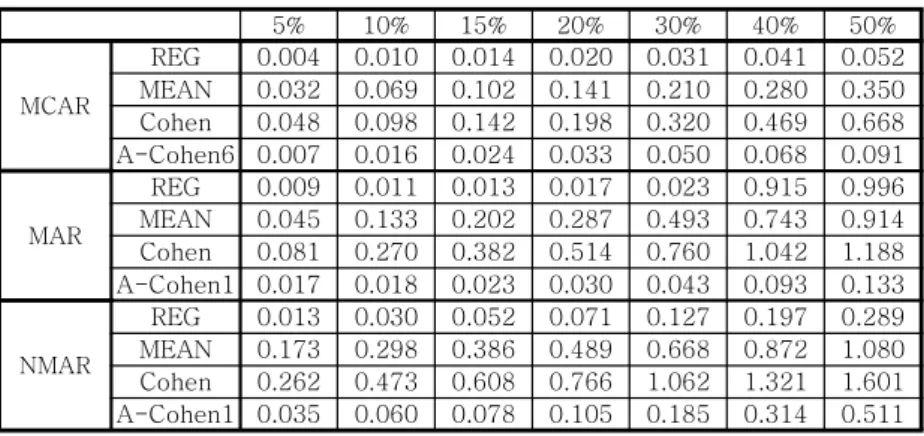
Simulation is performed under MCAR, MAR, and NMAR assumptions. Sepal length of Iris data is missing in the first simulation, petal length is missing in the second and of generated data is missing in the third. Table 3 shows detail information. With notes, 'depends on PL' means sepal length of Iris data is first sorted by petal length and then omitted as missing rate. This simulation design is referred by the literature of Allison(2000), Horton and Lipsitz(2001) and Scheffer(2002). The simulation using Iris data is done separately, because the distributions of sepal length and petal length have different shapes.
data mechanisms variable with
missing values notes
Iris
MCAR ・ SL ・ PL ・ missing randomly, each 1000 times MAR ・ SL ・ PL ・ depends on PL ・ depends on PW NMAR ・ SL ・ PL ・ depends on itself
Generated
MCAR ・ ・ missing randomly, each 1000 times
MAR ・ ・ depends on
NMAR ・ ・ depends on itself
<Table 3> Simulation missing mechanisms
(3) Missing rates
The simulation is done with seven types of missing rates, 5, 10, 15, 20, 30, 40, 50 percent, for each of the missing mechanisms and data.
A simulation was done to compare results of adjusted Cohen methods. We compared the imputation methods in terms of the mean and standard deviation of data and mean square error of imputed values.
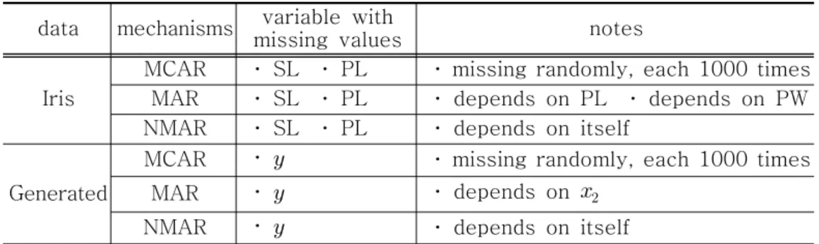
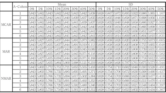
Table 4 and Table 5 presents the mean, standard deviation and MSE(mean square error) of adjusted Cohen methods of Iris sepal length data. In MCAR, adjusted Cohen6 has the best result - nearest mean, nearest standard deviation and smallest MSE. Also, in MAR and NMAR, adjusted Cohen1 gives the best result. Simulation of Iris petal length data and generated data were also performed and the results were similar to the result of Iris sepal length data. Therefore, in this study, we employed adjusted Cohen6 for MCAR and adjusted Cohen1 for MAR and NMAR.
(4) Imputation methods
Five imputation methods are used, which are multiple imputations using MCMC algorithm, regression imputation, mean imputation, Cohen method and adjusted Cohen method.
A-Cohen Mean SD
0% 5% 10% 15% 20% 30% 40% 50% 0% 5% 10% 15% 20% 30% 40% 50%
MCAR
1 5.843 5.842 5.843 5.842 5.842 5.843 5.842 5.838 0.828 0.847 0.872 0.895 0.922 0.986 1.065 1.167 2 5.843 5.842 5.842 5.841 5.840 5.839 5.837 5.835 0.828 0.835 0.846 0.858 0.871 0.908 0.956 1.026 3 5.843 5.842 5.842 5.842 5.841 5.841 5.839 5.837 0.828 0.832 0.840 0.848 0.858 0.886 0.927 0.989 4 5.843 5.842 5.843 5.843 5.842 5.843 5.842 5.840 0.828 0.830 0.834 0.838 0.845 0.866 0.898 0.950 5 5.843 5.842 5.843 5.842 5.842 5.843 5.842 5.841 0.828 0.828 0.829 0.832 0.836 0.851 0.877 0.922 6 5.843 5.842 5.843 5.842 5.841 5.843 5.842 5.841 0.828 0.819 0.814 0.809 0.805 0.804 0.810 0.831
MAR
1 5.843 5.827 5.835 5.837 5.844 5.891 5.973 5.962 0.828 0.838 0.826 0.820 0.808 0.755 0.673 0.665 2 5.843 5.827 5.835 5.837 5.844 5.891 6.019 6.113 0.828 0.838 0.826 0.820 0.808 0.755 0.665 0.648 3 5.843 5.827 5.835 5.837 5.844 5.916 6.045 6.089 0.828 0.838 0.826 0.820 0.808 0.739 0.631 0.600 4 5.843 5.827 5.835 5.837 5.844 5.945 6.071 6.116 0.828 0.838 0.826 0.820 0.808 0.718 0.612 0.582 5 5.843 5.827 5.835 6.004 5.844 5.945 6.071 6.168 0.828 0.838 0.826 0.820 0.808 0.718 0.612 0.589 6 5.843 5.827 5.835 5.864 5.900 5.998 6.121 6.219 0.828 0.838 0.826 0.797 0.761 0.675 0.573 0.544
NMAR
1 5.843 5.803 5.772 5.751 5.721 5.655 5.555 5.416 0.828 0.754 0.710 0.682 0.646 0.593 0.528 0.491 2 5.843 5.803 5.766 5.732 5.685 5.605 5.495 5.371 0.828 0.754 0.706 0.672 0.630 0.568 0.490 0.427 3 5.843 5.803 5.766 5.732 5.694 5.617 5.502 5.364 0.828 0.754 0.703 0.666 0.625 0.560 0.477 0.418 4 5.843 5.803 5.766 5.732 5.691 5.605 5.492 5.353 0.828 0.754 0.703 0.666 0.622 0.551 0.470 0.410 5 5.843 5.753 5.766 5.729 5.682 5.592 5.480 5.346 0.828 0.754 0.703 0.665 0.621 0.548 0.464 0.397 6 5.843 5.803 5.759 5.716 5.661 5.561 5.445 5.312 0.828 0.754 0.697 0.653 0.602 0.521 0.434 0.367
<Table 4> Mean and SD of adjusted Cohen methods
A-Cohen 5% 10% 15% 20% 30% 40% 50%
MCAR
1 0.027 0.061 0.091 0.128 0.212 0.318 0.462 2 0.015 0.033 0.051 0.070 0.116 0.174 0.251 3 0.012 0.027 0.041 0.057 0.094 0.139 0.203 4 0.011 0.024 0.036 0.051 0.082 0.120 0.173 5 0.009 0.019 0.029 0.041 0.065 0.095 0.136 6 0.007 0.016 0.024 0.033 0.050 0.068 0.091
MAR
1 0.017 0.018 0.023 0.030 0.043 0.093 0.133 2 0.017 0.018 0.023 0.030 0.043 0.133 0.213 3 0.017 0.018 0.023 0.030 0.064 0.157 0.199 4 0.017 0.018 0.023 0.030 0.080 0.184 0.231 5 0.017 0.018 0.023 0.030 0.080 0.184 0.273 6 0.017 0.018 0.034 0.056 0.125 0.246 0.346
NMAR
1 0.035 0.060 0.078 0.105 0.185 0.314 0.511 2 0.035 0.071 0.107 0.159 0.254 0.392 0.567 3 0.035 0.067 0.098 0.135 0.224 0.364 0.557 4 0.035 0.060 0.098 0.138 0.234 0.378 0.573 5 0.035 0.067 0.103 0.154 0.257 0.399 0.586 6 0.035 0.075 0.119 0.180 0.297 0.452 0.647
<Table 5> MSE of adjusted Cohen methods
4.2.2 Simulation results 4.2.2 Simulation results 4.2.2 Simulation results 4.2.2 Simulation results
Table 6 shows the mean and standard deviation when there are diverse missing ratio, under the various missing mechanisms. The first column represents the mean and standard deviations when the data are complete.
In common, as missing rate increases, standard deviations are decreased
seriously and means are also affected except for the MCAR assumption.
(1) The results of Iris Sepal length data
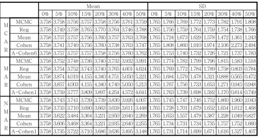
The mean, standard deviation and MSE of Iris sepal length data are represented in Table 7 and Table 8. Under MCAR, all of these methods estimate the true mean very well. Even at 50% missing, all means are within 1% of the target value. In the MAR
data 0% 5% 10% 15% 20% 30% 40% 50%
Iris SL
Mean
MCAR 5.843 5.843 5.843 5.842 5.841 5.843 5.843 5.843 MAR 5.843 5.882 5.950 6.004 6.069 6.212 6.367 6.477 NMAR 5.843 5.753 5.674 5.612 5.541 5.411 5.285 5.158 SD
MCAR 0.828 0.827 0.828 0.827 0.826 0.825 0.826 0.826 MAR 0.828 0.820 0.791 0.773 0.750 0.687 0.605 0.595 NMAR 0.828 0.738 0.680 0.643 0.600 0.535 0.459 0.392
Iris PL
Mean
MCAR 3.758 3.757 3.757 3.756 3.760 3.757 3.763 3.768 MAR 3.758 3.874 4.019 4.155 4.340 4.751 5.050 5.221 NMAR 3.758 3.622 3.484 3.364 3.221 2.950 2.640 2.269 SD
MCAR 1.765 1.724 1.673 1.629 1.578 1.472 1.361 1.243 MAR 1.765 1.725 1.666 1.601 1.478 1.064 0.732 0.670 NMAR 1.765 1.694 1.642 1.602 1.552 1.470 1.357 1.174
generated Mean
MCAR 11.044 11.043 11.043 11.048 11.044 11.044 11.041 11.050 MAR 11.044 11.355 11.609 11.827 12.080 12.528 13.009 13.412 NMAR 11.044 10.601 10.257 9.954 9.667 9.109 8.533 7.938 SD
MCAR 3.916 3.916 3.917 3.914 3.917 3.917 3.911 3.917 MAR 3.916 3.732 3.616 3.549 3.438 3.313 3.190 3.212 NMAR 3.916 3.473 3.234 3.068 2.932 2.706 2.490 2.302
<Table 6> Mean and SD of Iris SL, Iris PL and generated data
Mean SD
0% 5% 10% 15% 20% 30% 40% 50% 0% 5% 10% 15% 20% 30% 40% 50%
M C A R
MCMC 5.843 5.843 5.842 5.840 5.844 5.838 5.843 5.844 0.828 0.828 0.831 0.831 0.831 0.836 0.837 0.845 Reg 5.843 5.843 5.843 5.842 5.842 5.842 5.842 5.840 0.828 0.825 0.822 0.819 0.816 0.810 0.805 0.800 Mean 5.843 5.843 5.843 5.842 5.841 5.843 5.843 5.843 0.828 0.808 0.785 0.763 0.738 0.690 0.638 0.582 Cohen 5.843 5.835 5.835 5.842 5.841 5.834 5.843 5.833 0.828 0.847 0.872 0.895 0.923 0.987 1.066 1.168 A-Cohen6 5.843 5.842 5.843 5.842 5.841 5.843 5.842 5.841 0.828 0.819 0.814 0.809 0.805 0.804 0.810 0.831
M A R
MCMC 5.843 5.831 5.829 5.817 5.815 5.728 5.594 5.617 0.828 0.837 0.845 0.861 0.864 0.968 1.135 1.111 Reg 5.843 5.832 5.832 5.827 5.823 5.788 5.682 5.659 0.828 0.833 0.834 0.839 0.841 0.878 0.991 1.007 Mean 5.843 5.882 5.950 6.004 6.069 6.212 6.367 6.477 0.828 0.801 0.750 0.713 0.670 0.574 0.467 0.419 Cohen 5.843 5.874 5.942 6.004 6.069 6.205 6.367 6.470 0.828 0.840 0.834 0.837 0.838 0.821 0.781 0.842 A-Cohen1 5.843 5.827 5.835 5.837 5.844 5.891 5.973 5.962 0.828 0.838 0.826 0.820 0.808 0.755 0.673 0.665 N
M A R
MCMC 5.843 5.823 5.800 5.767 5.739 5.686 5.643 5.621 0.828 0.793 0.765 0.724 0.696 0.653 0.626 0.628 Reg 5.843 5.821 5.795 5.764 5.731 5.676 5.624 5.562 0.828 0.787 0.748 0.713 0.676 0.624 0.585 0.546 Mean 5.843 5.753 5.674 5.612 5.541 5.417 5.285 5.158 0.828 0.721 0.644 0.594 0.536 0.447 0.355 0.276 Cohen 5.843 5.746 5.667 5.612 5.541 5.411 5.285 5.154 0.828 0.756 0.716 0.696 0.671 0.640 0.593 0.555 A-Cohen1 5.843 5.803 5.772 5.751 5.721 5.655 5.555 5.416 0.828 0.754 0.710 0.682 0.646 0.593 0.528 0.491
<Table 7> Mean and SD of Iris SL data