In Pursuit of Low Carbon Cities : Understanding Limitations of ICLEI’s International Local Government Greenhouse Gas Emissions Protocol

(1)

In Pursuit of Low Carbon Cities: Understanding Limitations of ICLEI’s International Local Government Greenhouse Gas Emissions Protocol

Oh Seok Kim*

저탄소도시를 지향하며 -ICLEI 규약의 한계성 분석-

김오석*

Abstract : This article addresses potential errors in accounting greenhouse gas (GHG) emissions based on the International Council for Local Environmental Initiatives’ (ICLEI’s) International Local Government Greenhouse Gas Emissions Analysis Protocol (IEAP). The IEAP seems to provide practical guidelines for local governments so that they can measure their GHG emissions. The outcomes are immediately convertible for any national GHG inventory analysis when one is constructed based on the methodology drafted by Intergovernmental Panel on Climate Change. Further, it provides a societal foundation at the global level in order for local governments to collectively deal with ‘double-counting’ and ‘allocation’

problems. However, ICLEI’s IEAP overlooks two major issues: (1) the protocol does not consider carbon dioxide emissions due to burning biological fuel as a type of GHG emission; and (2) it overlooks the possibility of indirect double-counting when producing emission factors at the local level. Thus, the limitations must be fixed so that the local governments can measure their GHG emissions more precisely, while the accurate GHG inventory will ultimately support reducing the local governments’ emissions to mitigate anthropogenic climate change.

Key Words : carbon emission, greenhouse gas, biofuel, city, climate change

요약 :지방정부로 구성된 국제환경 협의회(ICLEI)는 범지구적 차원에서 기후변화를 완화시키기 위해 만들어

진 기구이다. 지방정부들은 ICLEI를 통해 각 정부가 배출하는 온실가스를 정확히 측정하고자 관련 규약을 만 들었다. 본 논문은 ICLEI 규약의 한계점을 지적한다. 온실가스배출관련 항목들을 지방정부관점에서 구분하 고, 또 국가차원에서 요구하는 항목들과 일치시킨다는 점에서 이 규약은 실용적이라 할 수 있다. 특히 ‘이중측 정’과 ‘탄소배출할당’ 문제를 해결할 수 있는 사회적 기반을 마련한 부분은 지방정부들이 기후변화에 적극적으 로 대응하고자 하는 의지로 해석할 수 있다. 하지만, 그 제한점은 다음과 같다. ‘생체연료연소에 의한 이산화탄 소배출’을 온실가스로 취급하지 않는 점과 ‘간접이중측정’을 간과한 점은 온실가스배출량의 정확한 측정을 저 해할 것으로 예상되며, 이들을 수정보완해야 지방정부들이 기후변화를 완화시키는데 있어 실제로 기여할 수 있을 것이다.

주요어 :탄소배출, 온실가스, 생체연료, 도시, 기후변화

* Ph.D. Candidate, Geography Doctoral Program, University of Southern California, Los Angeles, CA 90089, USA

Research Associate, Asian Institute for Energy, Environment and Sustainability, Seoul National University, Seoul, 151-921, Korea, [email protected]

(2)

1. Introduction

1) Problem statement

Climate change is one of the most serious threats the geopolitical world faces, and many scientists argue that anthropogenic greenhouse gas (GHG) emissions are responsible for such a global crisis (IPCC Working Group I, 2007). To protect human’s habitat, it appears to be crucial to mitigate the ongoing climate change, and one way to do so is by reducing GHG emissions to the atmosphere (IPCC Working Group III, 2007). It becomes, then, logical to account the current stage of GHG emissions accurately, first and foremost, because human society should know what kind of measure to take to reduce emissions and to successfully account and audit for the changes implemented.

On 19th of October 2012, the ‘Seoul Declaration of Local Governments on Energy and Climate Miti- gation’ was announced by Mayor of Seoul, on behalf of the World Mayors Council on Climate Change (WMCCC) and International Council for Local Environmental Initiatives – Local Governments for Sustainability (ICLEI). That is to say, the two global organizations will invest a lot effort to save city-wise energy consumption and GHG emissions (WMCCC and ICLEI, 2012). According to the World Health Organization, more than 50% people now live in urban areas at the global level, so it seems reasonable that more than 260 cities are willing to join such collective actions to reduce their emissions, while ICLEI’s protocols are designed to support measuring the cities’

carbon footprints. In the case of Korea, however, no studies have used ICLEI’s protocols, and this hardly makes sense given more than 90% of Korean citizens now live in urban areas (Kim, 2010); further, there are limited studies in Korean Geographical Society that talk about low carbon issues (Kim, 2010; Kwon

et al., 2010; Yu, 2010). Moreover, the country rest- lessly exports and imports many goods overseas while such trading has been the biggest momentum that has sustained its national economy ever since. Thus, there is a need to thoroughly understand GHG accounting protocols that are globally accepted and to maximize their use from Korean local governments’ perspective.

2) Scales of GHG emissions

The GHG accounting efforts may be better yet when those are done collectively at different scales (Angel et al., 1998; Kates et al., 1998). Angel et al. (1998) argue that at a local scale, it is quite common a summation of producers’ emissions and that of consumers’ emissions are not identical, where the producers’ emissions indicate the GHGs generated when producing goods, while the consumers’ emissions are measured when the goods are buried in landfills as waste, which apparently result GHG emissions. However, at the global scale, summations of producers’ and consumers’

emissions are pretty much identical. The mismatch at the local level is mainly because cities cannot always produce what they need for themselves so they have to rely on other cities’ goods and materials. That is, many goods and materials are consumed in the cities that do not produce such goods and materials; hence, this situation implies any climate change mitigation actions in urban areas should take place at the local level collectively, not at the mere ‘global’ level. Kates et al. (1998) also contend, “action to reduce greenhouse gases is never global, and despite much rhetoric is rare- ly national, but is mostly local (p280).” In other words, localized efforts to mitigate anthropogenic climate change must take the lead to collectively cope with the global crisis; thus, constructing accurate GHG inventories at different scales seems fundamental.

Numerous GHG accounting protocols have been used up to date in this context at different scales:

(3)

ranging from national level protocols, e.g., Intergov- ernmental Panel on Climate Change’s (IPCC’s) 2006 IPCC Guidelines for National Greenhouse Gas Inven- tories (IPCC, 2006), to product-level protocols, e.g., British Standard Institute (BSI) British Standards’

PAS 2050:2011 (BSI British Standards et al., 2011) or International Organization for Standardization’s (ISO’s) 14067 (ISO, 2011; ISO, 2010). Protocols by World Business Council for Sustainable Development (WBCSD) and World Resources Institute (WRI) are geared towards supporting GHG measurements of cooperates and/or their projects, while those of U.S.

Environmental Protection Agency (EPA) and Climate Registry in Northern America (CR) are designed to account emissions at the facility-level, e.g., factories (IPCC, 2006; ICLEI, 2009; WBCSD and WRI, 2010, 2005; Boston, 2007; The Climate Registry, 2008). Different scales of existing GHG accounting protocols are summarized in Table 1.

Table 1. Scale of GHG accounting protocols.

Organization Scale

IPCC National level

ICLEI State/city/community level WBCSD/WRI Corporate/project level

ISO Organization level

EPA Facility level

CR Facility level

ICLEI’s protocols are twofold: Local Government Operations Protocol (LGO) Version 1.1 (ICLEI, 2010) and International Local Government GHG Emissions Analysis Protocol (IEAP) Version 1 (ICLEI, 2009).

The former protocol supports a local government’s GHG inventory analysis as accurately as possible, while the latter protocol is rather about facilitating the global communication among local governments to promote their collective actions. In short, the IEAP is a streamlined version of the LGO, and by scarifying the

inventory’s accuracy the IEAP becomes more efficient in sharing information. It is also unique in a sense that the protocol is constituted with multiple spatial scales (Table 1). Accounting GHG emissions may seem like an easy and mundane task, but in fact, it is neither easy nor mundane, in particular when different spatial scales are involved. In addition, there are potential errors when urban GHG inventories are constructed based on the IEAP, especially the way the protocol treats carbon emissions is problematic. Thus, the present paper points out and explains the limitations of the IEAP so as to facilitate an accurate global communication among local governments.

2. Getting to Know Carbon Emissions

1) Greenhouse gases

GHGs are divided to two categories: (1) Kyoto Gases and (2) GHG Precursors. The Kyoto Gases refer to the major GHGs that have the most effective contribution to anthropogenic climate change, and these are mandated to be monitored, according to the Kyoto Protocol (UNFCCC, 1998). Whereas, the GHG Pre- cursors have a minor climate change impact compared to the Kyoto Gases so those are not accounted often in carbon offset projects (WBCSD and WRI, 2007). The Kyoto Gases include:

• Carbon dioxide (CO2),

• Methane (CH4),

• Nitrous oxide (N2O),

• Hydrofluorocarbons (HFCs),

• Perfluorocarbons (PFCs), and

• Sulphur hexafluoride (SF6).

As there are other environmental regulations which

(4)

mandate to document some of the GHGs for different purposes, it may be practically useful to stress such gases because the information may strengthen data availability when constructing a GHG inventory. The HFCs and PFCs are the substitutes for ozone-deplet- ing compounds (ODCs), and these are momentarily monitored by the Montreal Protocol; the protocol is an embodiment of intergovernmental efforts to prevent the ozone depletion in the stratosphere (UNEP, 2009).

Nitrogen oxide (NOx) is worth paying extra attention as well because many air pollution regulations include NOx as part of their lists due to its toxic attribute.

They have to be documented regardless of the climate change impact (WBCSD and WRI, 2007).

An inventory analysis may have to report its GHG profile in tonnes of carbon dioxide equivalent (tCO2e) because the Kyoto Gases have different levels of global warming potential (GWP), so there is a need for using a unified measurement that allows comparing varying climate change impacts of different GHGs. For example, CH4 can heat up the earth 21 times more ef- ficiently than CO2 in a given time period (usually 100 years). That is, if there is 1 tonne of methane in the atmosphere its greenhouse effect is actually equivalent to that of 25 tonnes of carbon dioxide, i.e., 25 tCO2e. In the case of ODC’s substitutes and SF6, they have larger GWPs than CO2 or CH4 (Table 2), but the amounts are overall relatively small. Thus as a whole, their climate change impacts are smaller than those of CO2

and CH4, and this is why understanding carbon emissions is indispensable to effectively mitigate climate change. The GWPs of the Kyoto Gases are presented in Table 2, while the values are originated from IPCC’s Second Assessment Report (SAR).

2) Carbon flux

In order to precisely understand and measure any carbon emissions, it is fundamental to grasp the full mechanism of carbon flux system. Carbon literally exists everywhere. Some exists in the atmosphere, while some other is embedded in wood and paper products that human frequently uses and disposes.

Carbon is also mobile. That is, it does not stay in a particular (carbon) pool, rather it moves around from one pool to another and to another endlessly.

When carbon is accumulated in a biomass, for instance, basically the carbon was transferred from the atmosphere to the biomass. In other words, this process could be rephrased as a carbon transfer from a carbon pool (i.e., the atmosphere) to another (i.e., the biomass). Hence from the biomass perspective, it ‘sequesters’ the carbon, while momentarily the carbon was ‘removed’ from the atmosphere.

This is why documents and reports produced and distributed by IPCC employ the terminology ‘carbon removal,’ while many other GHG accounting documents also use the term ‘carbon sequestration;’

they in fact indicate the identical direction of carbon flux. Besides, the biomass in this case is regarded as

‘carbon sink.’ Conversely, if the biomass ‘emits’ or

‘releases’ carbon to the atmosphere, the biomass is then considered ‘carbon source.’ Figure 1 visualizes the system of such carbon flux. Lastly, it is true that the atmosphere could be treated as a carbon source when a biomass becomes a carbon sink as those are coupled, but the reason that any GHG accounting documents do not explain such carbon flux from this Table 2. Global Warming Potential (GWP) values,

adapted from ICLEI (2009, p10).

GHG GWP

CO2 1

CH4 21

N2O 310

HFCs 140-11,700

PFCs 6,500-9,200

SF6 23,900

(5)

viewpoint is because human society’s ultimate goal is to reduce atmospheric carbon as much as possible, not the other way around.

3. Accounting Methodology

1) IPCC methodology

First and foremost, it is crucial to understand the IPCC methodology as many GHG accounting protocols depend on this (IPCC, 2006). Therefore, this section presents basic terminologies of the IPCC methodology that the IEAP often uses.

(1) Activity data and emission factor

The following equation is the most fundamental ap- proach when accounting any GHG emissions by the IPCC methodology:

Emissions = Activity Data×Emission Factor,

where ‘Activity Data’ indicates “[quantitative] information on the extent to which a human activity takes

place (p1.6),” while an ‘Emission Factor’ refers to the corresponding GHG emissions per unit activity; some popular ones are found in IPCC Emission Factor Da- tabase (IPCC, 2006). For example, gas or electricity bills are regarded as activity data as they show meter information or quantified measures of energy used.

Such information quantifies the associated human activities, such as energy use to cook food or transport goods. The emission factor, in this regards, indicates the amount of GHG generated when processing gas or producing electricity and consuming them for cooking or transporting. It is worth noting that the IEAP employs emission factors of IPCC’s SAR. ICLEI acknowledges the newer emission factors in IPCC’s Third or Fourth Assessment Reports are scientifi- cally more accurate than those of SAR, but ICLEI concludes using SAR’s emission factors has further advantage in facilitating communication among local governments.

(2) Tier

The IPCC methodology presents Tier concept in order to clarify different levels of methodological complexity, and different Tiers are introduced as follows:

Figure 1. System of carbon flux

(6)

• Tier 1 uses default emission factors provided in the IPCC methodology; country-specific activity data are preferable, but globally available data are often used, which are usually spatially and temporally coarse;

• Tier 2 requires higher spatio-temporal resolutions and more disaggregated activity data, and these are often based on country- or region-specific data sources, while emission factors are country-specific;

• Tier 3 needs to ref lect sub-national variation as well as interannual variability of an activity;

spatially explicit land-use activity data exemplify the complexity of this Tier; and thorough quality assurance and quality control (QA/QC) are mandated to assure the methodological accuracy.

The Tier 3 may provide greater certainty than the Tiers 1 or 2 only when it includes a sound QA/QC component. Spatially explicit, or Geographic In- formation Systems/Science based (GIS-based), data are considered Tier 3 since such spatial method can systematically track, for instance, land-use and land- cover change over time and portray the associated interannual variability of the local climate (IPCC, 2006). GIS, including remote sensing, plays a crucial role in this respect, namely data acquisition, management, visualization, and spatial analyses and modeling (Goodchild, 2003). The British Columbia Govern- ment’s Community Energy and Emission Inventory Initiative now intends to collect high resolution geore- ferenced data of GHG sources over time to construct a high quality GHG inventory at the state level (Boston, 2007).

2) Boundary

Unlike the IPCC methodology, the IEAP requires to account GHG emissions at two distinct jurisdictional levels: 1) organizational and 2) geopolitical

boundaries (ICLEI, 2009). By nature, specifying the two boundaries are not always straightforward, and this situation directly leads us to ‘allocation’ and ‘double-counting’ issues when accounting GHG emissions of a city, which will be discussed later in this paper.

The cumulative emissions of organizational and geopolitical boundaries are not added together, and they have to be accounted and reported separately (ICLEI, 2009, p45).

(1) Organizational boundary

The ‘organizational boundary’ indicates the direct jurisdiction of a local government at the facility level. That is, the boundary may not be identical to an administrative district per se. The concept actually includes any facilities, even though they are located outside the administrative district, that follow direct orders from the local government. Thus, emissions ris- ing from an organizational boundary must include all significant governmental assets and services, including contracted services and leased properties. All emissions associated with any governmental operations have to be accounted regardless of where those occur. This, as a result, enforces cities to document cross-regional GHG emissions that they are responsible for (ICLEI, 2009).

(2) Geopolitical boundary

The ‘geopolitical boundary’ is defined as “the physi- cal area or region over which a local government has jurisdictional authority (ICLEI, 2009, p10).” This is also regarded as a community-scale analysis, and this implies the boundary can be somewhat different from formal administrative districts. Once a geopolitical boundary is specified at a metropolitan scale, for instance, then it should include all possible emissions generated within the metropolitan region. A few ex- ceptions may be transportation and solid waste and wastewater treatments because vehicles often travel different communities and waste management facili-

(7)

ties could be located outside of the geopolitical boundary (ICLEI, 2009).

3) Scope

Scope embodies a perspective of life-cycle assessment (LCA), where the LCA is a main tool in Indus- trial Ecology to account all possible environmental debts that any production may generate as byproduct (Graedel and Allenby, 2003). The LCA is defined by the Society of Environmental Toxicology and Chemis- try (SETAC) as follows:

The life-cycle assessment is an objective process to evaluate the environmental burdens associated with a product, process, or activity by identify- ing and quantifying energy and material usage and environmental release, to assess the impact of those energy and material uses and releases on the environment, and to evaluate and implement opportunities to effect environmental improve- ments. The assessment includes the entire life cycle of the product, process or activity, encom- passing extracting and processing raw materials;

manufacturing, transportation, and distribution;

use/reuse/maintenance; recycling; and final disposal (Graedel and Allenby, 2003, p183).

The Scope is originated from WBCSD/WRI’s protocols to prevent double-counting, while this is also a big challenge in urban GHG inventory analyses.

That is to say, a city like Seoul, for instance, involves extremely complicated supply chains as it is the biggest national hub in terms of material flow in South Korea. The city also has a keen relationship with other adjacent cities, e.g., Incheon, because they are under the same metropolitan umbrella. Therefore, if a city accounts its GHG emissions without employing the concept of Scope, it would become very difficult to

clarify whether or not an emission source is accounted once or twice. Given this circumstance, ICLEI’s IEAP uses both ‘sector’ and ‘scope’ to avoid double-counting and also to later address allocation issues—who is responsible for a particular emission?; hence, each sector could be further classified to three scopes: from Scopes 1 to 3, and they are introduced as follow:

• Scope 1 indicates direct GHG emissions (except direct CO2 emissions from biomass combustion); for instance, fuel combustion and refrigerants’ leakage (i.e., fugitive emissions) are considered Scope 1;

• Scope 2 refers to indirect GHG emissions associ- ated with consumption of purchased electricity, heating or cooling; so this accounts emissions oc- curred when producing electricity, and gas for heating/cooling purpose;

• Scope 3 includes all indirect GHG emissions that are not part of Scopes 1 and 2; basically, it includes a full life-cycle inventory that has the largest system boundary, where a system boundary refers to a range of analysis when conducting an LCA;

GHG inventory reporting of a local government is preferred to include Scope 3 emissions according to ICLEI’ IEAP; the associated accounting method- ologies must be included and well explained; and

• Information item shows the items that are con- sidered emission-free, such as CO2 emissions from waste or biological fuel, wind farms, solar panels, etc.; documenting such items would present a more complete picture of communities’ energy use and emission patterns (ICLEI, 2009).

4) Allocation

ICLEI regards cities as consumers, and it thinks the consumers are responsible for any GHG emissions if those are associated with urban consumptions. This is why contracted services and leased properties must be

(8)

accounted although they are often considered Scope 3 emissions, while similar types of emissions are often omitted in other carbon offsetting projects (VCS, 2010). The term “demand-centered” by Ramaswami et al. (2008) exemplifies the very concept, where it refers to the activity data collection within a specific boundary.

5) Sector

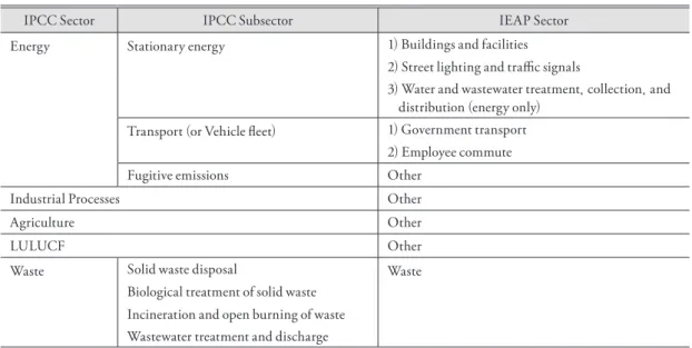
(1) Sectors for organizational boundary The IEAP provides numerous sectors for each boundary. The IEAP’s sectors are immediately convertible to IPCC’s sectors, which is reasonable for a practical reason as many countries are now mandated to report their national GHG inventory due to the Kyoto Protocol. Table 3 shows the relationship between the IPCC’s sectors and the IEAP’s sectors for the organizational boundary (ICLEI, 2009, p25). In short, the IEAP aggregates the IPCC’s fugitive emissions, industrial processes, agriculture, and Land-Use, Land-Use Change and Forestry (LULUCF) sectors

to its ‘other’ category, whereas stationary energy and transport sectors are divided to multiple categories.

The fugitive emissions refer to GHG releases from pressurized equipments in air conditioners or refrigera- tors due to leakage and any other unintended releases.

Table 4 summarizes GHG sources for the organizational boundary’s sectors. Each sector is further categorized to three scopes. The IEAP mandates to separately track and report municipal electricity and centralized heating/cooling that are supplied to the municipal grid systems. Those GHG sources are vul- nerable to double-counting since they could be also reported as Scope 2 emissions elsewhere. This does not include, however, municipal electricity and centralized heating/cooling that are not supplied to the municipal grid systems (ICLEI, 2009).

(2) Sectors for geopolitical boundary Sectors for the geopolitical boundary are rather unclear compared to those for the organizational boundary. For instance, the IPCC’s agricultural sector is divided to 1) ‘agricultural emissions’ and 2) ‘other,’ but

Table 3. IPCC sectors and IEAP sectors (organizational boundary), adapted from ICLEI (2009, p25)

IPCC Sector IPCC Subsector IEAP Sector

Energy Stationary energy 1) Buildings and facilities

2) Street lighting and traffic signals

3) Water and wastewater treatment, collection, and distribution (energy only)

Transport (or Vehicle fleet) 1) Government transport 2) Employee commute

Fugitive emissions Other

Industrial Processes Other

Agriculture Other

LULUCF Other

Waste Solid waste disposal Waste

Biological treatment of solid waste Incineration and open burning of waste Wastewater treatment and discharge

(9)

Table 4. Scope of IEAP sectors (organizational boundary)

IEAP Sector/Subsector Scope 1 Scope 2 Scope 3

Buildings and facilities Utility-delivered and decentral- ized fuel consumption;

Government owned utility- consumed fuel for electricity/

heat generation;

All stationary combustion sources not included in street- lights or water/wastewater sections.

Utility-delivered electricity/

heat/steam/cooling consumption.

Emissions from facilities operated by contracted businesses performing essential governmental services.

Street lighting and traffic signals Fuel used for lights that are not associated with a particular facility.

Utility-delivered electricity consumption.

Water/wastewater treatment,

collection, and distribution Fuel used in water/wastewater treatment, pumping, delivery, and disposal.

Government transport Tailpipe emissions from government owned and operated vehicles.

Electricity used by government owned electric vehicles.

Business and air travel.

Employee commute Tailpipe emissions from

employee’s commute.

Waste Solid waste generated by the government itself

Emissions from employee-generated solid waste, plus other solid waste if disposed of at a facility operated by the government.

Emissions from employee- generated solid waste, plus other solid waste if disposed of elsewhere.

Operation of solid waste

disposal sites Emissions from waste disposal sites when those are owned or operated by the government.

Operation of wastewater

treatment plants Emissions from wastewater, sewage, and industrial wastewater if the plant is owned or operated by the government.

Emissions from wastewater, sewage, and industrial wastewater if the plant has a contractual relationship with the government.

Other Fugitive emissions Emissions within the organizational boundary.

Industrial processes

(including product use) Emissions within the organizational boundary.

Agriculture Emissions from livestock and land management practices on farms owned or operated by the government.

LULUCF Significant biogenic carbon flux (either positive or negative).

(10)

neither of them is explained why they are divided to two nor how to account them separately. Table 5 shows the relationship between the IPCC’s sectors and the IEAP’s sectors for the geopolitical boundary (ICLEI, 2009, p32).

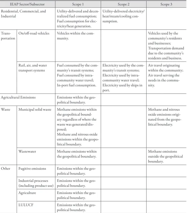
Table 6 summarizes GHG sources for the sectors of the geopolitical boundary. If data for residential, commercial, and industrial are not available separately, it is allowed to combine them as a whole and report the outcome, but extra caution is needed when comparing such outcome with other cities’ GHG inventory analyses. In the case of LULUCF sector, when data are fairly incomplete then it should be reported as an information item rather than a sector. Also, it is important to acknowledge the difference between waste generated and waste disposed: The ‘waste generated’ is “the gross amount of waste produced in the community,” while the ‘waste disposed’ is “the net amount of waste following the effects of any diversion (e.g., recycling or reuse) efforts (ICLEI, 2009, p39).”

Air travel and international shipping are major GHG sources. By nature, a large portion of emissions occurs outside a geopolitical boundary; hence, it is

highly controversial to allocate or assign the emissions to a specific geopolitical boundary or two. In addition, airports, seaports, and marinas in general serve multiple geopolitical boundaries. In the case of Incheon International Airport, citizens from Seoul, Incheon, Suwon, etc. use the airport to travel abroad, while on the other hand Seoul citizens may also use Kimpo Air- port to travel East Asian countries nearby, e.g., China.

Port of Busan, which is one of the largest ports in the world, encounters the same challenge as it functions as a national gateway in terms of material flow. Emissions associated with the operations of airports, seaports, and marinas should not be accounted as transportation. They should be reported with other sectors such as commercial electricity use. When a government owns any of airplanes, ships, airports, seaports, and marinas, then one must be reported under the organizational boundary.

6) Indicator

Comparing multiple cities in terms of GHG emissions is more than just comparing numbers. Many

Table 5. IPCC sectors and IEAP sectors (geopolitical boundary), adapted from ICLEI (2009, p32)

IPCC Sector IPCC Subsector IEAP Sector

Energy Stationary energy 1) Residential

2) Commercial 3) Industrial

Transport Transportation

Fugitive emissions Other

Industrial Processes Other

Agriculture 1) Agricultural emissions

2) Other

LULUCF Other

Waste Solid waste disposal Waste

Biological treatment of solid waste Incineration and open burning of waste Wastewater treatment and discharge

(11)

other factors must be factored in such as city size, location, population, business level, climatic condi- tions, etc. The IEAP refers to these items as “indicators (ICLEI, 2009, p46),” they must be taken account when normalizing GHG emissions is necessary for any

comparison. Studies that compare multiple global cities include indicators, namely population, total land area, density of urbanized area, heating degree days, and per capita income (Kennedy et al., 2010, 2009).

Table 6. Scope of IEAP sectors (geopolitical boundary)

IEAP Sector/Subsector Scope 1 Scope 2 Scope 3

Residential, Commercial, and

Industrial Utility-delivered and decen- tralized fuel consumption;

Fuel consumption for electricity/heat generation.

Trans- portation

On/off-road vehicles Vehicles within the community.

Vehicles used by the community’s residents and businesses;

Transportation demand due to the community’s residents and business.

Rail, air, and water transport systems

Fuel consumed by the community’s transit systems;

Fuel consumed by intra- community water travel;

In-port fuel consumption.

Electricity used by the community’s transit systems;

Electricity used by intra- community water travel;

Electricity used by ships in port.

Air travel originating within the community;

Air travel serving the needs in the community.

Agricultural Emissions Emissions within the geopolitical boundary.

Waste Municipal solid waste Methane emissions within the geopolitical boundary regardless of where the waste was generated/disposed;

Methane and nitrous oxide emissions within the geopolitical boundary.

Methane and nitrous oxide emissions originated from the geopolitical boundary.

Wastewater Methane emissions within the geopolitical boundary.

Methane emissions outside the geopolitical boundary.

Other Fugitive emissions Emissions within the geopolitical boundary.

Industrial processes (including product use)

Emissions within the geopolitical boundary.

Agriculture Emissions within the geopolitical boundary.

LULUCF Emissions within the geopolitical boundary.

(12)

4. Potential Accounting Errors

1) Biological fuel

According to the IEAP, CO2 emissions due to burning biological fuel is not considered GHG emis- sions unless an inventory includes agriculture and/

or LULUCF sectors. That is because ICLEI contends CO2 emissions from burning biological fuel must be regarded as part of “natural” carbon cycle unlike CO2

emissions from burning fossil fuel. Presumably, its intention is to provide extra incentives to those who frequently use biofuel, which is usually considered more environmentally friendly than fossil fuel, or to those who incinerate CH4 in landfills instead of merely releasing CH4 which has a higher GWP than the burned CH4 (i.e., CO2). ICLEI rationalizes its

“natural” carbon cycle by telling us how an apple ma- tures and how it eventually releases its carbon stock to the atmosphere when it decays (ICLEI, 2009, p8).

Because of this rationale, the IEAP does not mandate to account the CO2 generated from burning biological fuel. However, this instruction is misleading and may produce serious errors. That is, by design, the IEAP ignores the science of carbon flux and the associated time dimension. More specifically, ICLEI’s illustration of its

“natural” carbon cycle ignores soil and time factors; an apple never evaporates in the natural circumstance, yet it decays in soil and its carbon stock will reside there for a certain amount of time and will be released in future. It is true that soil carbon is often omitted even in the agriculture and LULUCF sectors, although it is by far the largest terrestrial carbon pool on the planet, primarily because its measurement is more challeng- ing than measuring other carbon pools. This does not justify, however, omitting the soil completely when ra- tionalizing a carbon cycle. In sum, CO2 emissions due to burning biological fuel must be distinguished from

the real natural CO2 emissions simply due to their different paces of carbon release to the atmosphere.

Such varying paces are crucial, for instance, when conducting a dynamic modeling to simulate carbon flux (Gower, 2003; Running and Gower, 1991); that is, different paces will produce different carbon emission outcomes. Besides, there is another reason why time has to be factored in when quantifying GHG emissions and estimating their climate change impacts. It was mentioned previously noting that a GHG can have multiple GWP values. That is, the GWP values in this paper are calibrated based on a 100 year time window;

in other words, if a series of GWP uses a 200 year time frame, for example, then the new GWP profile will have different numbers, and hence, this will result different GHG inventory outcome even with the identical activity data. In short, figures that do not consider such temporal dimensions are problematic. Thus, burning biological fuel must not be accounted as a mere information item because it is not emission-free;

in fact, this should be documented with greater details as we do not know for sure its true GWP.

2) Emission factor and ‘indirect’

double-counting

Transparent system boundaries (i.e., the concept of Scope) should be applied when generating emission factors to support further transparency in a GHG inventory analysis. The emission factors of Scope 1 is relatively straightforward to determine, but those of Scopes 2 and 3 are quite unclear to specify because their system boundaries can vary substantially when producing an emission factor, and they are not always clearly mentioned. The “hybrid method” by Ramaswa- mi et al. (2008) is a good example that addresses such issue. Even though the authors collected activity data within a specific geopolitical boundary, when producing their own emission factors they conducted cross-

(13)

regional analyses to assure better accuracy and transparency. For instance, if some gasoline is produced in a different city and later the fuel is transported to another city, the cross-regional travel distance will be taken into account if the hybrid method is used. As shown above, without considering transparent system boundaries of emission factors, it is likely to indirectly double-count climate change impacts of GHGs which might lead to a false GHG inventory analysis. Thus, it appears to be reasonable to clearly document their system boundaries when generating the emission factors of Scopes 2 and 3.

5. Conclusion

The IEAP provides practical guidelines for local governments so that they can accurately measure their emissions, and the outcomes are immediately convertible for any national GHG inventory analysis, when one is constructed based on the IPCC methodology.

It also provides a societal mechanism in order for the local governments to collectively deal with ‘double- counting’ and ‘allocation’ issues. However, ICLEI’s IEAP overlooks two major issues: (1) the protocol does not consider carbon dioxide emissions due to burning biological fuel as a member of greenhouse gases; and (2) it overlooks a possibility of indirect double-counting, which is different from an ordinary double-counting.

Such omission is partly because ICLEI lacks in sci- entific understanding in carbon flux and life-cycle analysis; as a result, the IEAP may provide distorted incentives to the local governments that intensively rely on biofuel, while its environmental impacts are still controversial (Johnson, 2009). Thus, the limitations must be fixed so that the local governments can more accurately measure their GHG emissions, so as to reduce the emissions to mitigate anthropogenic cli-

mate change.

Acknowledgements

The author acknowledges the support of ‘Forest Sci- ence & Technology Research Projects’ (Project No.

S210912L010110) provided by the Korea Forest Ser- vice and HSBC Fellowship of Center for Sustainable Cities at University of Southern California.

References

Angel, D. P., Attoh, S., Kromm, D., Dehart, J., Slocum, R., and White, S, 1998, The drivers of greenhouse gas emissions: What do we learn from local case studies? Local Environment, 3(3), 263-77.

Boston, A., 2007, Best Practices and Better Protocols, British Columbia Ministry of Environment, Community Energy and Emissions Inventory Working Group, and Holland Barrs Planning Group, British Co-, British Co-British Co- lumbia, Canada.

BSI British Standards, Carbon Trust, and Department for Environment Food and Rural Affairs, 2011, PAS 2050:2011 - Specification for the assessment of the life cycle greenhouse gas emissions of goods and ser- vices, BSI British Standards, London.

CR, 2008, General Reporting Protocols for the Voluntary Reporting Program, Version 1.1, Th e Climate Reg-The Climate Reg- istry, Los Angeles.

Goodchild, M. F., 2003, Geographic Information Science and Systems for Environmental Management, An- nual Review of Environment and Resources, 28(1), 493-519.

Graedel, T. E. and Allenby, B. R., 2003, Industrial Ecology, 2nd Edition, Prentice Hall, Upper Saddle River.

ICLEI, 2009, International Local Government GHG Emis- sions Analysis Protocol, International Council for Local Environmental Initiatives (ICLEI) - Local

(14)

Governments for Sustainability, Bonn.

ICLEI, 2010, Local Government Operations Protocol for the quantification and reporting of greenhouse gas emis- sions inventories, International Council for Local Environmental Initiatives (ICLEI) - Local Gov- (ICLEI) - Local Gov-ICLEI) - Local Gov-) - Local Gov-Local Gov- ernments for Sustainability, Bonn.

IPCC, 2006, 2006 IPCC Guidelines for �ational Green- IPCC Guidelines for �ational Green-IPCC Guidelines for �ational Green- house Gas Inventories, Institute for Global Envi-Institute for Global Envi- ronmental Strategies for the Intergovernmental Panel on Climate Change (IPCC), Kanagawa.

IPCC Working Group I, 2007, Contribution of Working Group I to the �ourth Assessment Report of the In- to the �ourth Assessment Report of the In-to the �ourth Assessment Report of the In- tergovernmental Panel on Climate Change 2007, Cambridge University Press, Cambridge and New York.

IPCC Working Group III, 2007, Contribution of Working Group III to the �ourth Assessment Report of the Intergovernmental Panel on Climate Change 2007, Cambridge University Press, Cambridge and New York.

ISO, 2010, Carbon footprint of products - Part 1: �uan-Part 1: �uan- 1: �uan-1: �uan-: �uan-�uan- tification, International Standards Organisation (ISO), Geneva.

ISO, 2011, Carbon footprint of products - Requirements and guidelines for quantification and communication, International Standards Organisation (ISO), Ge- (ISO), Ge-ISO), Ge-), Ge-Ge- neva.

Johnson, E., 2009, Goodbye to carbon neutral: Getting biomass footprints right, Environmental Impact Assessment Review, 29(3), 165-168.

Kates, R. W., Mayfield, M. W., Torrie, R. D., and Witcher, B., 1998, Methods for estimating greenhouse gases from local places, Local Environment, 3(3), 279-297.

Kennedy, C., Steinberger, J., Gasson, B., Hansen, Y., Hill-, C., Steinberger, J., Gasson, B., Hansen, Y., Hill-C., Steinberger, J., Gasson, B., Hansen, Y., Hill-., Steinberger, J., Gasson, B., Hansen, Y., Hill-Steinberger, J., Gasson, B., Hansen, Y., Hill-, J., Gasson, B., Hansen, Y., Hill-J., Gasson, B., Hansen, Y., Hill-., Gasson, B., Hansen, Y., Hill-Gasson, B., Hansen, Y., Hill-, B., Hansen, Y., Hill-B., Hansen, Y., Hill-., Hansen, Y., Hill-Hansen, Y., Hill-, Y., Hill-Y., Hill-., Hill-Hill- man, T., Havranek, M., Pataki, D., Phdungsilp, A., Ramaswami, A., and Mendez, G. V., 2010, Methodology for inventorying greenhouse gas emissions from global cities, Energy Policy, 38, 4828-4837.

Kennedy, C., Steinberger, J., Gasson, B., Hansen, Y., Hill-, C., Steinberger, J., Gasson, B., Hansen, Y., Hill-C., Steinberger, J., Gasson, B., Hansen, Y., Hill-., Steinberger, J., Gasson, B., Hansen, Y., Hill-Steinberger, J., Gasson, B., Hansen, Y., Hill-, J., Gasson, B., Hansen, Y., Hill-J., Gasson, B., Hansen, Y., Hill-., Gasson, B., Hansen, Y., Hill-Gasson, B., Hansen, Y., Hill-, B., Hansen, Y., Hill-B., Hansen, Y., Hill-., Hansen, Y., Hill-Hansen, Y., Hill-, Y., Hill-Y., Hill-., Hill-Hill- man, T., Havranek, M., Pataki, D., Phdungsilp,

A., Ramaswami, A., and Villalba Mendez, G., 2009, Greenhouse gas emissions from global cit-, Greenhouse gas emissions from global cit-Greenhouse gas emissions from global cit- ies, Environmental Science & Technology, 43(19), 7297-7302.

Kim, H.-C., 2010, A Comparative Analysis on the Levels of Local Governments against Climate Change in the World - Focused on ICLEI Members, Korean Journal of Local Government Studies, 14(3), 373- 390 (in Korean).

Kim, J. -H., 2010, ‘Green Growth’ and the Possible Con-, J. -H., 2010, ‘Green Growth’ and the Possible Con-J. -H., 2010, ‘Green Growth’ and the Possible Con-. -H., 2010, ‘Green Growth’ and the Possible Con-H., 2010, ‘Green Growth’ and the Possible Con-., 2010, ‘Green Growth’ and the Possible Con-2010, ‘Green Growth’ and the Possible Con-, ‘Green Growth’ and the Possible Con-Green Growth’ and the Possible Con-’ and the Possible Con-and the Possible Con- tribution of Geomorphologic Studies, Journal of the Korean Geographical Society, 45(1), 75-94 (in Korean).

Kwon, Y.-W., Wang, K.-I., and Yu, S.-C., 2010, On Low- Carbon Green Waterfront Cities, Journal of the Korean Geographical Society, 45(1), 1-10 (in Ko-45(1), 1-10 (in Ko-(1), 1-10 (in Ko-1), 1-10 (in Ko-), 1-10 (in Ko-1-10 (in Ko--10 (in Ko-10 (in Ko- (in Ko-in Ko- rean).

Ramaswami, A., Hillman, T., Janson, B., Reiner, M., and Thomas, G., 2008, Policy Analysis: A Demand- Centered, Hybrid Life-Cycle Methodology for City-Scale Greenhouse Gas Inventories, Environ- mental Science & Technology, 42(17), 6455-6461.

UNEP, 2009, The Montreal Protocol on Substances that Deplete the Ozone Layer, United Nations Environ-United Nations Environ- ment Programme (UNEP), Nairobi.

UNFCCC, 1998, Kyoto Protocol to the United �ations

�ramework Convention on Climate Change, United Nations Framework Convention on Climate Change (UNFCCC), Kyoto.

VCS, 2010, Approved VCS Module VMD0007 Version 1.0 REDD Methodological Module: Estimation of base-: Estimation of base-Estimation of base- line carbon stock changes and greenhouse gas emis- sions from unplanned deforestation �BL-UP� Sec- �BL-UP� Sec-BL-UP� Sec--UP� Sec-UP� Sec-� Sec-Sec- toral Scope 14, Verified Carbon Standard (VCS), Washington, DC.

WBCSD and WRI, 2005, The Greenhouse Gas Protocol:

The GHG Protocol for Project Accounting, World Business Council for Sustainable Development (WBCSD) and World Resources Institute (WRI), Conches-Geneva and Washington, DC.

WBCSD and WRI, 2007, Measuring to Manage: A Guide to Designing GHG Accounting and Reporting Pro-

(15)

grams, World Business Council for Sustainable Development (WBCSD) and World Resources Institute (WRI), Conches-Geneva and Washing- (WRI), Conches-Geneva and Washing-WRI), Conches-Geneva and Washing-), Conches-Geneva and Washing-Conches-Geneva and Washing--Geneva and Washing-Geneva and Washing- ton, DC.

WBCSD and WRI, 2010, Product Accounting and Re-, 2010, Product Accounting and Re-2010, Product Accounting and Re-, Product Accounting and Re-Product Accounting and Re- porting Standard (Draft for stakeholder review), World Business Council for Sustainable Develop- ment (WBCSD) and World Resources Institute (WRI), Conches-Geneva, and Washington, DC.

WMCCC and ICLEI, 2012, 2012 Seoul Declaration of Local Governments on Energy and Climate Mitigation, World Mayors Council on Climate Change (WMCCC) and ICLEI Global Executive Committee, Seoul.

Yu, K.-B., 2010, Geography: A Portal to Green Growth, Journal of the Korean Geographical Society, 45(1), 11-25 (in Korean).

교신: 김오석, 미국 남가주대학교 지리학 박사과정(이메 일: [email protected])

Correspondence: Oh Seok Kim, Geography Doctoral Pro-: Oh Seok Kim, Geography Doctoral Pro-Oh Seok Kim, Geography Doctoral Pro-, Geography Doctoral Pro-Geography Doctoral Pro- gram, University of Southern California, Los Angeles, CA 90089, USA (e-mail: [email protected])

Recieved �ovember 8, 2012 Revised �ebruary 12, 2013 Accepted �ebruary 18, 2013