Single-axis Hardware in the Loop Experiment Verification of ADCS for Low Earth Orbit Cube-Satellite

JPNT 6(4), 195-203 (2017)

https://doi.org/10.11003/JPNT.2017.6.4.195

Copyright © The Institute of Positioning, Navigation, and Timing

JPNT

Journal of Positioning, Navigation, and Timing

http://www.ipnt.or.kr Print ISSN: 2288-8187 Online ISSN: 2289-0866

1. INTRODUCTION

A payload in a cube satellite is generally dependent on the mission purpose. Seoul National University GNSS Laboratory satellITE (SNUGLITE) has the following payloads: dual- frequency(L1/L2) GPS receivers, boom structure and fine magnetometer to observe the Earth magnetic field (Kim et al.

2016). As reference sensors for the Attitude Determination and Control System (ADCS), sun sensors and magnetometer are used, while as a rate sensor, gyroscopes are mainly used (Ni & Zhang 2011). Coarse sun sensors have accuracy within 5-10° in general, whereas expensive fine sun sensors have a better accuracy within 0.01°. SNUGLITE uses an inexpensive photodiode-type coarse sun sensor as a sensor for attitude determination sensor, and also employs three- axis magnetometer and three-axis gyroscope for attitude

Single-axis Hardware in the Loop Experiment Verification of ADCS for Low Earth Orbit Cube-Satellite

Minkyu Choi, Jooyoung Jang, Sunkyoung Yu, O-Jong Kim, Hanjoon Shim, Changdon Kee

^†

Mechanical and Aerospace Engineering and the Institute of Advanced Aerospace Technology, Seoul National University, Seoul 151-744, Korea

ABSTRACT

A 2U cube satellite called SNUGLITE has been developed by GNSS Research Laboratory in Seoul National University. Its main mission is to perform actual operation by mounting dual-frequency global positioning system (GPS) receivers. Its scientific mission aims to observe space environments and collect data. It is essential for a cube satellite to control an Earth-oriented attitude for reliable and successful data transmission and reception. To this end, an attitude estimation and control algorithm, Attitude Determination and Control System (ADCS), has been implemented in the on-board computer (OBC) processor in real time. In this paper, the Extended Kalman Filter (EKF) was employed as the attitude estimation algorithm. For the attitude control technique, the Linear Quadratic Gaussian (LQG) was utilized. The algorithm was verified through the processor in the loop simulation (PILS) procedure. To validate the ADCS algorithm in the ground, the experimental verification via a single axis Hardware-in-the-loop simulation (HILS) was used due to the simplicity and cost effectiveness, rather than using the 3-axis HILS verification (Schwartz et al. 2003) with complex air-bearing mechanism design and high cost.

Keywords: ADCS, EKF, LQG, sensor calibration, single-axis HILS

determination sensor (Jang et al. 2016).

Estimation algorithms using attitude determination sensors can be typically divided into statistical estimation methods using quaternion such as QUEST (Ran et al. ‎2014), REQUEST, extended Kalman filter (EKF), and deterministic estimation methods including TRIAD algorithm. The TRIAD algorithm is used as the estimation algorithm during the initial stage, and then EKF is used to estimate the attitude of satellite. For the reference coordinate, a magnetic field model of the International Geomagnetic Reference Field (IGRF)-12 provided by the International Association of Geomagnetism and Aeronomy (IAGA), and DE405 solar model in the NASA Jet Propulsion Laboratory (JPL) were used.

In addition, a magnetorquer using magnet moment and reaction wheel or control moment gyro (CMG) are used as an actuator for control. Since the reaction wheel or CMG employs a motor, they consume more power than the magnetorquer. Furthermore, since an additional actuator is needed for moment dumping, three-axis magnetorquer was used in this study due to the low consumption, lightweight, and good control reliability. For the control algorithm, the Received July 21, 2017 Revised Aug 17, 2017 Accepted Aug 18, 2017

†

Corresponding Author E-mail: [email protected]

Tel: +82-2-888-2069 Fax: +82-2-876-6649

196 JPNT 6(4), 195-203 (2017)

https://doi.org/10.11003/JPNT.2017.6.4.195

Linear Quadratic Gaussian (LQG) was used to generate a control gain in real time.

To develop a cube satellite, generally, the following steps are needed: first, an algorithm is designed through Software in the Loop Simulation (SILS) that verifies the algorithm in terms of software simulation. Next, the algorithm is implemented directly in the processor on-board computer (OBC) to verify the ADCS algorithm of the actual flight model (FM) through the Processor in the Loop Simulation (PILS) in real time. Finally, the ADCS algorithm is experimentally verified by simulating the space environment to validate the attitude estimation and control performance as well as the algorithm through the Hardware in the Loop Simulation (HILS). In the HILS verification, attitude estimation and control performance are verified through experimental procedure using air-bearing-based HILS simulator that is mechanically complex and has high design cost for three- axis attitude determination and control (Schwartz et al.

2003). Through this process, the ADCS algorithm in the cube satellite is finally designed and verified.

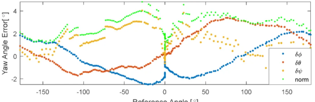
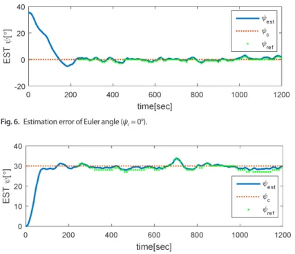
In this paper, PILS that is implemented in actual OBC is discussed; and lower cost and more practical single-axis HIL experimental verification, in contrast with the HILS verification process using air-bearing, was presented (Ure et al. 2011). In particular, actual payload sensors should be used. Thus, a study on the sensors error modeling and compensation is also conducted.

2. ADCS ALGORITHM

2.1 Coordinate Frames

In this study, a number of coordinate systems are used.

The Earth-centered inertial (ECI) coordinate system is a

coordinate system that represents a position of one point in the space based on the origin in the center coordinate system of the Earth mass. In the ECI coordinate system, the Earth's equatorial plane is set to X and Y axes. The X-axis refers to the Vernal equinox; the Z-axis a vertical line in the North Pole direction in the XY plane; and the Y-axis an axis that is perpendicular to the X and Y axes. Next, the Earth- centered Earth Fixed (ECEF) coordinate system is used, in which the X-axis of the ECI frame is fixed in the Greenwich meridian direction and thereby is rotated around the Earth's rotation axis. This can be seen in Fig. 1, in which the Z-axis is defined as the Earth's center direction from the mass center of the satellite, and the Y-axis is defined as an outer product between Z-axis and velocity direction of the satellite. The X-axis refers to an outer product between the Y and X axes.

In addition, the body frame that represents an attitude of the satellite is defined by the Euler angle as shown in Fig. 2.

As described in the Introduction, the solar position model (JPL DE405) calculates a solar position through the ECI coordinate, and the Earth's magnetic field model (IGRF- 12) is a model for the Earth's magnetic field. Thus, the ECEF coordinate system belongs to this (Kim 2015).

2.2 Attitude Determination Based on EKF

For the EKF to estimate the attitude state of the cube satellite, a linear Kalman filter, which linearized a non-linear system at the nominal point, was used (Jang 2016). Eq. (1) expresses the attitude information of the satellite. x̂(t) refers to quaternions, ω̂(t) an angular rate, and b̂(t) a gyro bias. The superscript of each variable expresses an estimate.

2.2 Attitude Determination Based on EKF

For the EKF to estimate the attitude state of the cube satellite, a linear Kalman filter, which linearized a non-linear system at the nominal point, was used (Jang 2016). Eq. (1) expresses the attitude information of the satellite. ˆ( ) x refers to quaternions, t

^ω

^{ˆ ( )}

^t

an angular rate, and b ˆ( )t a gyro bias. The superscript of each variable expresses an estimate.

 

 

 

0 1 2 3

1 2 3

1 2 3

10 1

ˆ ˆ( )

ˆ ˆ

ˆ( ) ( ) ,

ˆ ( ) ˆ

T T T

q q q q t

t t

t b b b

  



  

 

   

  

 

q q

x ω ω

b b ₍₁₎

The kinematics equation of quaternion can be notated as it is divided into quaternion ˆ ( )

t

q

and angular velocity

^ω

^{ˆ ( )}

^t

as presented in Eq. (2).

1 1

ˆ ( ) ( ( )) ( ) ˆ ˆ ( ( )) ( ) ˆ ˆ

2 2

t  t t  t t

q Ω ω q Ξ q ω

(2)

1 2 3

1 3 2

2 3 1

3 2 1 4 4

0 ( ) 0

0 0

  

  

  

  

_

  

 

  

 

   

  

 

Ω ω  

1 2 3

0 3 2

3 0 1

2 1 0 4 3

q q q

q q q

q q q

q q q

_

  

 

  

 

   

  

 

Ξ q

The non-linear equation of the state variable is presented in Eq. (3), which is specified in detail in Eq. (4).

             

ˆ t  ˆ , t t  t , t ~ N 0,

x f x u w w Q ₍₃₎

   

 

 

1

1 ˆ ( ) ( ) ˆ

ˆ( ) 2

ˆ ˆ ˆ

ˆ( ), ( ) ( ) ( ) ( ) ( ) ( ( )) ( )

ˆ ( ) 1 ˆ( ) ( )

BLB

k Bmeas D

bias

t t t

f t t t t t t t t t

t t t





 

 

     

     

                              

Ω ω q

q 0

x u w ω w I u B ω Iω η

b b η

(4) In Eq. (4), ( ) u refers to the control input, t B

^Bmeas

refers to the measurement of magnetic field in the body frame, and ( )t w represents the Gaussian-distributed white noise. In addition, the space model with external disturbance considered gravity gradient torque and torque generated due to air friction and solar radiation wind as the covariance matrix (Q) as presented in Eq. (5).

   

       

 

4 4 4 3 4 3

2 2 2

3 4 3 3 3 3

2

3 4 3 3 3 3

, ~ 0, ,

k D k GGT SRP AD

bias k

RRW

t t t N

t

  



  

  

  

 

   

   

                

0 0 0

0

w η w Q Q 0 I 0

η 0 0 I ₍₅₎

(1)

Fig. 1. ECI, ECEF, local, body frame in space.