Feasibility of Using Prior Information about Predicted Item Difficulty in Increasing the Accuracy of Item Parameter Estimation and IRT Equating

2009, Vol. 12, No. 1, pp. 103～122

Feasibility of Using Prior Information about Predicted Item Difficulty in Increasing the Accuracy

of Item Parameter Estimation and IRT Equating

Yi, Hyun Sook (Assistant Professor, Konkuk University)

≪ SUMMARY ≫

For item banking or computerized adaptive testing to be successful, it is of vital importance to ensure the accuracy of item parameter estimation, especially when calibration needs to be conducted with the limited number of examinees for security reasons. This study investigated whether judgmental information about item difficulty would improve the accuracy of parameter estimation when used as prior information. Performance of using predictions of judges with various degrees of accuracy was evaluated in terms of item parameter invariance as well as effects on test equating, with reference to performances of other estimation methods under various simulation conditions. The findings of this study suggest that using priors based on judgmental information may increase the accuracy of b-parameter estimation and test equating in a considerable amount, unless predictions about item p-values are extremely inaccurate. The effects were even more obvious for the 1PL model and for smaller sample sizes. In estimating a-parameters and overall equating results for larger sample sizes, mixed results were found for the superiority of using judgmental information as priors.

Key words : Predicted item difficulty, Bayesian estimation, Prior information, Invariance of parameter estimation, IRT Equating

Ⅰ. Introduction

It is a typical practice in a large-scale testing program that new items are periodically added to

an existing item pool after item parameters of the new items are tried-out and calibrated. The

fact that new items should be exposed to a group of examinees before items are operationally used makes it an imperative role for test developers to keep test security to a maximum degree, usually by controlling for the number of examinees exposed to pre-test items as smallest as possible. This practice, however, may cause another serious problem threatening the stability of item parameter estimation, which is also a critical issue for an item banking or computerized adaptive testing to be successful. It is generally accepted that a sample size of 200 examinees is sufficient to obtain stable item parameters of the one parameter logistic (1PL) IRT model (Wright

& Stone, 1979), while much larger sample sizes (e.g. 1,000 examinees) are needed for the three parameter logistic (3PL) IRT model (Reckase, 1979). Since using smaller sample sizes than those suggested in the literature for estimating item parameters of pre-test items may result in inaccurate parameter estimation and undesirable results in equating, trade-offs should be made between stability in parameter estimation and test security when determining optimum sample sizes for pre-testing try-out items.

In addition to the consideration with regard to the sample size, one needs to choose a statistical procedure that provides the most accurate estimation under a given sample size.

Research has been conducted to find a statistical procedure that could increase the precision of parameter estimation. Several researchers have demonstrated that Bayesian estimation procedures tend to produce more accurate estimation compared to other estimation procedures and thus, need smaller sample sizes than others to achieve the same level of accuracy (Hambleton &

Swaminathan, 1985; Lim & Drasgow, 1990; Mislevy, 1987; Skaggs & Stevensen, 1989; Swaminathan, Hambleton, Sireci, Xing, & Rizavi, 2003). In determining prior distributions for Bayesian estimation, researchers have suggested to use additional information about characteristics of test items or examinees, that are not directly related to statistical properties of items (Kim & Huh, 2008), and obtained favorable results. For example, Mislevy (1987) suggested to use collateral information of test items (e.g. item format, content) or examinees (e.g. educational background) using Bayesian methods in estimating item parameters. Stout, Ackerman, Bolt, Froelich, and Heck (2003) recently explored the usefulness of an IRT-based collateral information approach to improve pretest item calibration. Also, Swaminathan, Hambleton, Sireci, Xing, & Rizavi (2003) illustrated that Bayesian estimation based on judgmental information about item difficulty was more effective in improving the accuracy of estimation compared to other estimation methods.

However, there is another line of research showing that accuracy is adversely affected when a Bayesian prior is mis-specified (Harwell & Janosky, 1991; Seong, 1990).

A couple of high-stakes testing programs in South Korea routinely take the procedure of

gathering judgmental information about item difficulty in the process of test development. Since empirically testing new items is very limited in high-stakes tests for security concerns, a group of item writers and/or item reviewers take a couple of rounds of predicting item difficulty for each item based on their past experiences and knowledge about contents and examinee performances.

As a way of exploring effective statistical procedures for ensuring the accuracy of parameter estimation given limited sample sizes, this study was designed to investigate whether incorporating judgmental information about item difficulty by item writers and/or reviewers with various degrees of accuracy in prediction would improve the precision of parameter estimation when used as prior information for Bayesian estimation procedures. Performance of using priors based on subject matter expert(SME)'s prediction about item difficulty was examined and compared with other estimation methods under various sample sizes for calibration as well as psychometric models.

This study can be seen as an extension of the work by Swaminathan et al. (2003), with differences being that this study used simulated data sets under various simulation conditions and evaluated the results at the test level as well as at the item level.

Ⅱ. Methods and Procedures

1. Simulation Factors

In order to investigate whether the judgmental information about item difficulty improves the

accuracy of parameter estimation when used as prior information for Bayesian estimation procedures,

three factors that might affect the estimation of item parameters were considered: (1) psychometric

models (1PL vs. 3PL), (2) sample sizes for calibration (100; 200; 500; 1,000; and 3,000), and (3)

forms of prior information based on degrees of accuracy in predicting item difficulty (priors based

on observed item difficulty; priors based on predicted item difficulty with 10% discrepancy; priors

based on predicted item difficulty with 20% discrepancy; priors based on predicted item difficulty

with 30% discrepancy; priors based on N(0,1); and no prior). The first two factors were chosen

because the choice of psychometric models and sample sizes for calibration is known to be an

important factor affecting the accuracy of parameter estimation. The last factor was considered to

see whether varying degrees of accuracy in prediction about item difficulty would make differences

in accuracy of parameter estimation and equating when used as prior information and to get

information about how accurate a prediction should be in order to obtain parameters with acceptable

level of accuracy.

For the simulation factor of psychometric models, 3PL model was first chosen because it was considered as the most accurately reflecting the nature of multiple choice items by incorporating guessing behavior of examinees, and 1PL model was also chosen because the model was considered to require the smallest sample size to achieve a certain degree of accuracy among three IRT models. For the condition of sample sizes, wider ranges of the sample sizes were considered compared to the study by Swaminathan et al. (2003) in order to observe the performance of estimation under optimal conditions as well as less-than-optimal conditions. 1,000- and 200-examinee conditions were chosen first because the former was the minimum requirement for the 3PL model and the latter for the 1PL model, respectively (Chang, Hanson, and Harris, 2001). And then, 500- and 100- examinee conditions were also considered to observe gradual patterns of accuracy in parameter estimation when less than optimal sample sizes are used for 3PL and 1PL models, respectively. Lastly, 3,000-examinee conditions were chosen to represent the situation where sample sizes would not be an issue in calibration of any IRT models.

For the last simulation factor, various forms of sample-based prior information about item

difficulty parameter (b-parameter) based on different degrees of accuracy in predicting item

difficulty were considered. First, degrees of accuracy in predicting item difficulty were diversified

ranging from the perfect prediction where the predicted difficulty equals to the observed difficulty

to the prediction with gradually increasing discrepancy between the predicted and observed

difficulty. In order to determine the levels of accuracy in prediction, typical patterns in judgment

of item difficulty in terms of degrees of accuracy were explored. For this purpose, a subject

consisting of 30 dichotomously-scored items was chosen from a nationwide testing program that

employs judgmental processes for obtaining item information. The judgmental processes applied in

this testing program usually take the following procedures. Subject matter experts (i.e. item writers

and/or item reviewers) who participate in the process of test development make judgments about

item difficulty for each item based on their past experiences and knowledge about contents and

examinee performances individually. And then, they take a couple of rounds of discussions until

they reach to an agreement. Information about both SME's ratings on predictive item difficulty

and the actual item difficulty is available for this subject in the form of percentages of correct

responses. After examining 10 alternate forms randomly selected from those administered within

the past 5 years to find the general pattern of discrepancies between the predicted and the

observed item difficulty, it was found that the absolute magnitude of the discrepancy between the

predicted and the observed item difficulty was ranging from the minimum of 1.07 to the

maximum of 25.41, having the mean of 10.44. Therefore, 10%, 20%, and 30% of discrepancy between the predicted and the observed difficulty, which represent small, medium, and large degrees of discrepancy, respectively, were considered as conditions for simulation. Situations where item parameter estimation was based on sample-free priors of N(0,1) or classical approach without prior information were also considered and compared with other forms of prior information.

Factors were fully crossed, leading to a total of 60 simulation conditions. Although the simulation factors considered in this study may not entirely capture the whole picture of the testing practices, they were regarded as the essential conditions of calibration of item parameters that could possibly affect the accuracy of item parameter estimation. All simulation conditions were replicated for 100 times.

2. Data Generation and Simulation Procedures

True item parameters for generating data sets for the simulation study were obtained from a data set in public domain (Kolen and Brennan, 2004, p. 192). Three item parameters (a-, b-, and c-parameters) for the 36 items of Form X served as true item parameters. Item response data were generated using the three item parameters for each of the 36 items, and the 3PL IRT model was used to generate examinee responses to represent realistic responses to multiple-choice items.

First, a set of ability parameters, θ, for each of 3,000 simulees were generated assuming that the ability is distributed as the standard normal distribution. Then, a dichotomous response (Uij) for item i and simulee j was generated by comparing a value of the random number R in the interval [0,1] to the population value of the correct response probability Pij by the following rule:

if R≤Pij, then Uij=1, otherwise Uij=0, where Pij was calculated by the 3PL IRT model based on the three true item parameters and the examinee’s ability θ. Item response data for 3,000 simulees were first generated and those for sample sizes of 1,000, 500, 200, and 100 were made by randomly selecting the corresponding number of simulees out of the item responses for the 3,000 simulees. This is to reflect the real context where a certain portion of examinees are randomly selected from a larger pool of examinees for calibration purposes.

After item response data were generated, item parameters were estimated using 1PL and 3PL

models, respectively. For each psychometric model, 6 forms of prior information described in the

previous section were used for estimating item parameters. In estimating b-parameters, the prior

distribution of the b-parameter of each item was assumed to be distributed as a normal

distribution with the mean of the predicted item difficulty under various degrees of accuracy and

the standard deviation of 1. However, since judges' predictions are typically made in the form of percentage of correct responses (i.e. item p-value), scale transformation was needed beforehand because prior distributions of item difficulty parameter is represented as the scale of the b-parameter. Specifically, item p-values under various simulation conditions were first calculated for each item based on simulated item responses. These values were then transformed to the scale of IRT b-parameters based on the approximation proposed by Tucker (Swaminathan et al., 2003):

b

= U( a

-a

U

+a

U

) ( 1 - a

U

+a

U

) ,

where _{U = p - 2} , _a

_{= 2.5101} , _a

_{= 12.2043} , _a

_{= 11.2502} , _a

_{= 5.8742} , _a

_{= 7.9587} . The reason for choosing this transformation over other alternative transformation methods was because a normal prior was used for estimating b-parameters. After each p-value was transformed to the scale of the b-parameter, the scale of the transformed b-parameters was then adjusted to that of the true b-parameters used to generate data sets by applying linear regression. This is to resolve the problem of scale indeterminacy. The slope and the intercept found from the linear regression were applied to the scale transformation procedures under six simulation conditions to place all item parameters on the common scale. Transformed b-parameters were truncated to be placed within the range of -4 to +4 to eliminate unrealistic cases.

Prior distributions for the first simulation condition (priors based on observed difficulty;

‘observed p' hereafter) were assumed to be distributed as the normal distribution with the mean of the transformed p-values actually observed from the simulated data. In order to represent the second simulation condition (priors based on predicted difficulty with 10% discrepancy; ‘10%

discrepancy' hereafter), 10% of discrepancy of prediction was added to or subtracted from the predicted p-values and then scale transformation was made to set the scale of the b-parameters.

Prior distributions for the b-parameters were assumed to be distributed as the normal distribution

with the mean of the transformed b-parameters and the standard deviation of 1. Priors based on

predicted difficulty with 20% discrepancy (‘20% discrepancy' hereafter) and those based on

predicted difficulty with 30% discrepancy (‘30% discrepancy' hereafter) were determined in a

similar manner. Performance of item parameter estimation under the simulation conditions

described above was compared to the performance under priors based on N(0,1) and that of no

prior distribution. BILOG-MG (Zimowski, Muraki, Mislevy, & Bock, 1996) was used for

calibration using default options except for using the priors for the item difficulty parameter

estimation. In estimating item discrimination or guessing parameters for the 3PL model, priors

typically used in the procedure of estimating these two parameters were used, because judgmental information about these parameters were unavailable and the focus of this paper was to observe the effects of using judgmental information about item difficulty in accuracy of parameter estimation. The prior distribution for the a- parameters was taken as the log-normal distribution with the mean of 0 and the standard deviation of 1, and that of the c-parameters was taken as the beta distribution with the mean of 0.2 and standard deviation of 0.0095.

3. Equating

In order to observe whether the consequences of using inaccurate item parameter estimation have considerable effects on examinee scores, IRT true-score equating based on the 3PL model was conducted for each simulation condition. Item parameters of the Form X and Form Y used for simulation were considered as the true item parameters of the new form and the base form, respectively (Kolen and Brennan, 2004, p. 192), and these parameters were used to find the true equating relationships. Performance of equating based on estimated item parameters under various simulation conditions was evaluated with reference to the ‘true’ equating relationships established from the true item parameters from Form X and Form Y. The computer program PIE (Hanson &

Zeng, 1995) was used for the IRT true-score equating.

4. Evaluation Criteria

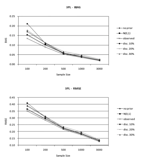
To evaluate the extent to which item parameter invariance is ensured under the 60 simulation conditions, two indices BIAS and RMSE (Root Mean Squared Error) were calculated at the item level to summarize the differences between the true item parameters and the estimated item parameters under each simulation condition. These indices are defined as

BIAS ₌ ∑

r = 1

(p

- p

) R and

RMSE ₌ ∑

r = 1

(p

- p

)

R ,

where R denotes the number of replications, p

denotes an estimate of a generic item parameter estimated at the r

replication, and p

denotes the true parameter of interest. These indices were first calculated for each item over 100 replications, and then averaged over 36 items.

To measure the overall performance of equating, another two indices that summarize the

differences between the estimated score equivalent and the score equivalent based on true item parameters were used. These indices are defined as

BIAS-T ₌ ∑

N i = 1

(ES

-TS

) N and

RMSE-T ₌ ∑

N i = 1

(ES

-TS

)

N ,

where ES represents the estimated score equivalent, TS represents the true score equivalent, and N represents the number of items.

Ⅲ. Results

1. Effects on Item Parameter Estimation

First of all, in order to explore the feasibility of using judges' ratings about item difficulty as

prior information in improving the accuracy of parameter estimation, accuracy of item parameter

estimation was evaluated at the item level. Average BIAS and RMSE indices under various

simulation conditions estimated using 1PL and 3PL models are summarized in Tables 1 and 2,

respectively. Bold-faced numbers indicate the smallest BIAS or RMSE among six forms of prior

distributions under each sample size, and italicized numbers indicate the largest BIAS or RMSE

among them. The average BIAS and RMSE indices obtained under the 1PL and the 3PL model

are represented in Figures 1 and 2, respectively. In general, all estimates of BIAS and RMSE

indices decreased as sample sizes increased, and the differences in performances among forms of

prior information increased as the sample size decreased. BIAS and RMSE indices estimated

under the 3PL model were markedly smaller than those for the 1PL model, implying that the

3PL model reflected the response patterns of multiple choice items more accurately. All BIAS

indices were positive, indicating that item parameters were overestimated.

<Table 1> Average BIAS and RMSE of Parameter Estimates Under the 1PL Model

Criterion Prior Distribution Sample Size

100 200 500 1,000 3,000

BIAS

No Prior 0.4551 0.4093 0.3856 0.3849 0.3764

N(0,1) 0.4324 0.4012 0.3832 0.3838 0.3760

Observed p 0.4092 0.3891 0.3782 0.3812 0.3751

Predicted p with 10% Discrepancy 0.4162 0.3915 0.3794 0.3819 0.3754 Predicted p with 20% Discrepancy 0.4168 0.3931 0.3801 0.3822 0.3755 Predicted p with 30% Discrepancy 0.4289 0.3976 0.3816 0.3829 0.3757

RMSE

No Prior 0.6169 0.5715 0.5438 0.5350 0.5263

N(0,1) 0.5961 0.5636 0.5411 0.5339 0.5260

Observed p 0.5807 0.5523 0.5362 0.5311 0.5250

Predicted p with 10% Discrepancy 0.5851 0.5575 0.5388 0.5326 0.5255 Predicted p with 20% Discrepancy 0.5854 0.5581 0.5391 0.5329 0.5256 Predicted p with 30% Discrepancy 0.5920 0.5608 0.5401 0.5334 0.5258

Patterns of relative performance among various simulation conditions were somewhat different between the estimates under the 1PL model and those under the 3PL model. As shown in Table 1 and Figure 1, the average BIAS and RMSE indices of b-parameter estimates of the 1PL model were smallest for the condition of the ‘observed p' and greatest for the condition of the ‘no prior' for all sample sizes being considered. Conditions with the ‘10% discrepancy', ‘20% discrepancy', and ‘30% discrepancy' followed the condition with the ‘observed p' in this order, and all conditions having the priors based on predicted item difficulty performed better than conditions having the priors of N(0,1) and those without prior information. These patterns were consistent for both BIAS and RMSE indices. This indicates that parameter estimation using priors based on judges’ ratings about item difficulty is likely to have more accurate estimates than other estimation methods. The fact that even with the largest discrepancy between the actual p-value and the predicted p-value as large as 30% performed better than estimations based on N(0,1) or without prior information corroborates this statement.

Differences in performances among forms of prior distributions decreased as the sample size increased, with non-distinguishable differences for the sample sizes greater than 1,000. For the sample size of 200, which is considered to be the minimum requirement for the 1PL model, the differences of both BIAS and RMSE indices among various prior distributions were fairly large.

For the sample size of 100, differences among prior distributions were even more obvious. This

implies that the choice of an estimation method may yield quite different parameter estimates under the condition of small sample sizes, which may cause non-ignorable influences on scoring.

[Figure 1] Average BIAS & RMSE of b-parameter Estimates Under the 1PL Model

On the other hand, as can be seen from Table 2 and Figure 2, somewhat inconsistent patterns were observed for the three item parameters estimated under the 3PL model. In the case of b-parameter estimation, it is consistent with the results estimated under the 1PL model that the condition with the ‘observed p' produced the most accurate results than other conditions, but performances of estimation under other conditions were inconsistent across sample sizes and also different for the BIAS and RMSE indices. For the sample sizes of 100 and 200, which may be extremely small to get stable estimates under the 3PL model, the conditions with ‘10%

discrepancy' and ‘30% discrepancy' tend to perform much worse than other conditions, although

the conditions with N(0,1) and no priors still did not perform better than those with ‘observed p' or ‘20% discrepancy'. These patterns were similar for BIAS and RMSE indices. This might be due to the fact that estimation error is too large for the conditions of 100 and 200 sample sizes to accurately estimate item parameters under the 3PL model regardless of the estimation methods.

However, with sample sizes greater than or equal to 500, stability of estimation seems to be at an acceptable level and the patterns of performance among forms of prior information were fairly consistent over sample sizes and for both BIAS and RMSE indices. Conditions of ‘10%

discrepancy' and ‘20% discrepancy' produced the second and the third smallest estimation errors among the six forms of prior information, while the ‘30% discrepancy' condition produced the most inaccurate estimation. Conditions with no priors and N(0,1) consistently performed worse than the conditions of ‘10% discrepancy' and ‘20% discrepancy' for sample sizes over 500. These findings imply that incorporating judges’ ratings as prior information seems to have positive effects in improving the accuracy of the b-parameter estimation over other methods of estimation in situations where using relatively small sample sizes is inevitable. Even for much smaller sample sizes than those required for estimating item parameters with stability, the results from this study imply the feasibility of using judgmental information about item difficulty as a prior information for estimating b-parameter in producing more accurate results if judges' predictions are fairly accurate (i.e. within 20% of discrepancy).

However, in the case of the a-parameter estimation, prior information based on N(0,1) distribution produced the smallest BIAS and RMSE indices, while the priors based on predicted p-values with 10% discrepancy showed the largest BIAS and RMSE indices under all sample sizes being considered. Although priors based on the predicted p-values with 20% and 30%

discrepancy produced smaller BIAS and RMSE indices compared to the results based on no prior

information, it may not be legal to state that estimation based on judgmental information about

item difficulty parameters also increases the accuracy of estimation of item discrimination

parameters, because priors based on observed p-values and predicted p-values with only 10% of

discrepancy performed worse than other conditions. This result might be due to the fact that

estimation of the item discrimination parameter is influenced by estimation of other parameters

such as examinee ability as well as the item difficulty. In the case of c-parameter estimation,

BIAS and RMSE indices remained approximately the same across all simulation conditions. This

result might be also due to the fact that the guessing parameter estimate is the function of

estimates of other parameters such as examinee ability and item discrimination as well as the

item difficulty.

<Table 2> Average BIAS and RMSE of Parameter Estimates Under the 3PL Model

Criterion Prior Distribution Sample Size

100 200 500 1,000 3,000

BIAS a

No Prior 0.1156 0.0890 0.0692 0.0418 0.0237

N(0,1) 0.0517 0.0354 0.0327 0.0171 0.0124

Observed p 0.1100 0.0847 0.0671 0.0408 0.0230

Predicted p with 10% Discrepancy 0.1689 0.1344 0.0890 0.0501 0.0252 Predicted p with 20% Discrepancy 0.0672 0.0498 0.0410 0.0254 0.0158 Predicted p with 30% Discrepancy 0.0600 0.0380 0.0331 0.0179 0.0120

b

No Prior 0.1693 0.1111 0.0586 0.0388 0.0204

N(0,1) 0.1533 0.1012 0.0594 0.0422 0.0233

Observed p 0.1340 0.0897 0.0526 0.0352 0.0186

Predicted p with 10% Discrepancy 0.2108 0.1079 0.0555 0.0389 0.0207 Predicted p with 20% Discrepancy 0.1521 0.0988 0.0582 0.0418 0.0229 Predicted p with 30% Discrepancy 0.1775 0.1118 0.0662 0.0483 0.0264

c

No Prior 0.0054 0.0052 0.0045 0.0035 0.0022

N(0,1) 0.0048 0.0046 0.0041 0.0034 0.0023

Observed p 0.0050 0.0047 0.0042 0.0033 0.0021

Predicted p with 10% Discrepancy 0.0053 0.0048 0.0041 0.0033 0.0021 Predicted p with 20% Discrepancy 0.0044 0.0043 0.0038 0.0033 0.0022 Predicted p with 30% Discrepancy 0.0049 0.0048 0.0043 0.0037 0.0025

RMSE a

No Prior 0.2994 0.2520 0.1953 0.1506 0.0968

N(0,1) 0.2764 0.2288 0.1749 0.1364 0.0906

Observed p 0.3036 0.2516 0.1936 0.1491 0.0956

Predicted p with 10% Discrepancy 0.3424 0.2886 0.2101 0.1538 0.0954 Predicted p with 20% Discrepancy 0.2821 0.2327 0.1753 0.1382 0.0905 Predicted p with 30% Discrepancy 0.2845 0.2361 0.1783 0.1389 0.0901

b

No Prior 0.3902 0.3112 0.2274 0.1839 0.1307

N(0,1) 0.3639 0.2943 0.2265 0.1879 0.1364

Observed p 0.3502 0.2835 0.2163 0.1761 0.1260

Predicted p with 10% Discrepancy 0.4085 0.3034 0.2213 0.1830 0.1308 Predicted p with 20% Discrepancy 0.3631 0.2912 0.2245 0.1866 0.1347 Predicted p with 30% Discrepancy 0.3872 0.3071 0.2372 0.1970 0.1408

c

No Prior 0.0656 0.0647 0.0605 0.0539 0.0430

N(0,1) 0.0618 0.0609 0.0586 0.0535 0.0438

Observed p 0.0627 0.0615 0.0582 0.0520 0.0417

Predicted p with 10% Discrepancy 0.0657 0.0634 0.0590 0.0530 0.0424

Predicted p with 20% Discrepancy 0.0606 0.0598 0.0570 0.0527 0.0429

Predicted p with 30% Discrepancy 0.0639 0.0629 0.0600 0.0551 0.0445

[Figure 2] Average BIAS and RMSE of b-parameter Estimates Under the 3PL Model

2. Effects on IRT Equating

In order to examine whether the degree to which item parameter estimation is inaccurate would affect scores of examinees at the test level, IRT true-score equating was conducted using item parameters obtained from 3PL model under various simulation conditions being explored in this study. The results were compared with reference to the ‘true’ equating relationship obtained from true item parameters of Form X and Form Y used for generating data sets.

Table 3 presents the average BIAS-T, RMSE-T, and the number of discrepant score equivalents

of IRT true-score equating with reference to the ‘true' equating relationship. Average BIAS-T was

computed by averaging the discrepancies between the ‘true’ score equivalent and unrounded

raw-to-raw score equivalent for each item and RMSE-T was computed by getting standard deviation of the squared sum of the discrepancies. After the unrounded raw-to-raw score conversion was established for all score points, score equivalents were rounded to the nearest integer, to reflect real testing contexts, and the number of discrepant score equivalent with reference to the rounded score equivalent obtained from the ‘true’ score conversion was computed. Bold-faced numbers indicate the smallest BIAS or RMSE among six forms of prior distributions under each sample size, and italicized numbers indicate the largest BIAS or RMSE among them.

<Table 3> BIAS-T, RMSE-T, and the Number of Discrepant Score Equivalents of IRT True Score Equating Under the 3PL Model

Sample

Size Prior Distribution BIAS-T RMSE-T No. of Discrepant

Score Equivalents

100

No prior 0.0327 0.3537 10

N(0,1) 0.0265 0.4044 12

Observed p 0.0322 0.3184 8

Predicted p with 10% Discrepancy 0.0428 0.2599 9

Predicted p with 20% Discrepancy 0.0262 0.4034 11

Predicted p with 30% Discrepancy 0.0033 0.4454 14

200

No prior 0.0172 0.2636 7

N(0,1) 0.0256 0.2823 8

Observed p 0.0120 0.2465 6

Predicted p with 10% Discrepancy 0.0178 0.2560 7

Predicted p with 20% Discrepancy 0.0220 0.2894 7

Predicted p with 30% Discrepancy 0.0121 0.2979 8

500

No prior -0.0276 0.2196 6

N(0,1) -0.0082 0.2080 5

Observed p -0.0267 0.2108 6

Predicted p with 10% Discrepancy -0.0389 0.2208 5

Predicted p with 20% Discrepancy -0.0079 0.2156 7

Predicted p with 30% Discrepancy -0.0161 0.2201 7

1,000

No prior -0.0405 0.1693 5

N(0,1) -0.0256 0.1446 5

Observed p -0.0391 0.1634 5

Predicted p with 10% Discrepancy -0.0413 0.1733 5

Predicted p with 20% Discrepancy -0.0354 0.1603 5

Predicted p with 30% Discrepancy -0.0331 0.1578 5

3,000

No prior -0.0402 0.1172 2

N(0,1) -0.0339 0.1080 2

Observed p -0.0387 0.1130 2

Predicted p with 10% Discrepancy -0.0402 0.1180 2

Predicted p with 20% Discrepancy -0.0382 0.1153 2

Predicted p with 30% Discrepancy -0.0378 0.1164 3

As can be observed from the table, in general, RMSE-T and the number of discrepant score equivalents decreased as the sample size increased, meaning equating results become more accurate under larger sample sizes. Whereas, BIAS-T indices shifted from positive to negative values as the sample size increased, meaning that equated score equivalents were overestimated when estimation was based on smaller sample sizes and underestimated when estimation was based on larger sample sizes. By examining the RMSE-T indices and the number of discrepant score equivalents, it seems that performance of equating based on three parameters estimated from different forms of prior information is somewhat different from the performance of parameter estimation at the item level. For sample sizes less than or equal to 500, equating results based on item parameters calibrated using priors based on observed p-values and those based on predicted p-values with 10% of discrepancy performed fairly well compared to other conditions, while equating results based on predicted p-values with 30% of discrepancy produced the largest equating errors. This suggests that using prior information based on judgmental information about item difficulty may increase the accuracy of equating at the test level with the relatively small sample sizes, unless the predicted p-values do not apart from the actual p-values in a great deal.

However, for sample sizes greater than or equal to 1,000, RMSE-T indices were smallest for the condition with N(0,1) and largest for the condition with ‘10% discrepancy', although the number of discrepant score equivalents based on rounded equated scores were nearly the same regardless of the estimation methods. For these sample sizes, performances of ‘observed p', ‘20%

discrepancy', and ‘30% discrepancy' were better than those without prior information, but this may not entirely suggest that incorporating prior information based on judges’ ratings could increase the accuracy of test equating results in all cases.

Ⅳ. Conclusions and Discussion

The feasibility of IRT equating or the validity of examinee scores obtained from equating

results primarily depends on the degree to which item parameters are calibrated with accuracy. In

situations where very limited number of examinees is only available or using small sample sizes

is inevitable in item calibration, choosing and employing an estimation method that may produce

the most accurate results is of vital importance. The present study examined the effects of using

prior information about item difficulty based on judges’ ratings on the accuracy of item parameter

estimation and the IRT true-score equating, by comparing results based on various prior distributions using different sample sizes under 1PL and 3PL IRT models.

This study showed that when the 1PL model was used for parameter estimation, using priors based on judgmental information produced obviously more accurate parameter estimation compared to estimations without incorporating prior information or using N(0,1) distribution as a prior for all sample sizes being explored. The effects were more obvious as the sample size decreased. For the 3PL model, however, different patterns were observed for the three item parameter estimates.

For the b-parameter estimation, using judgmental information about item difficulty as a prior information improved the accuracy of item parameter estimation if judges' predictions do not apart from the actual p-values in a great deal, while we have less confidence in stating that this is also true for estimation of a-parameters. At the test level, equating results based on item parameters calibrated using predicted p-values produced relatively accurate equating results compared to those without using any prior information or N(0,1) distribution with smaller sample sizes, while results for the larger sample sizes do not entirely support the superiority of estimation based on priors using judges' ratings. In fact, equating results based on rounded score equivalents were nearly the same across all estimation methods for larger sample sizes.

Overall, the findings of this study suggest that using priors based on judgmental information may increase the accuracy of item parameter estimation and test equating compared to other prior distributions when small sample sizes are used for item calibration, and therefore, may reduce the possible errors associated with examinee scores that might be caused by inaccurate estimation unless the prediction about p-values is extremely inaccurate. This observation was more obvious for the 1PL model than 3PL model especially for smaller sample sizes such as those less than or equal to 500. For example, performance of priors based on predicted p-values with 10%

discrepancy using 100 examinees marked almost as same as performance of estimates without prior information using 200 examinees. However, it should be noted that increasing sample size was the more influential factor than the choice of a psychometric model or prior information, and this observation was consistently made for all simulation conditions being considered in this study.

This suggests that increasing sample sizes will be the most reasonable choice in increasing the accuracy of the parameter estimation, if doing so can be achieved without other practical concerns.

However, if limiting sample sizes is inevitable for any practical reasons, incorporating judgmental information in parameter estimation may be an alternative choice that will have similar effects as using larger sample sizes for calibration.

The findings of this study might be especially useful in the context of high-stakes tests in our

country where statistical properties of items cannot be obtained before a test is operationally administered and the extremely high security concerns often hinder measurement practitioners from employing relatively new testing practices such as item banking or computerized adaptive testing.

Since gathering judgmental information about item statistics is typically incorporated in the process of developing nationwide high-stakes tests, this information can be used in calibration without extra costs. In other cases, however, it might be costly to recruit experienced judges, train them, and gather accurate judgmental information about item difficulty. Nevertheless, if limiting sample sizes for calibration is a critical issue for security concerns, employing prior information based on judges’ ratings about item difficulty can be a reasonable option that may produce accurate estimation with reduced item exposure rate.

There are a couple of limitations of this study, which lead to suggestions for future research.

First, since the 3PL model was used to generate response data in simulation process, there is a possibility that situations might have been favorable to the 3PL model than to the 1PL model.

Future studies comparing the performance of these two psychometric models based on data generated from the 1-PL model might provide corroborating evidence to the findings of this study.

Second, this study explored effects of using judgmental information about item difficulty in estimating item parameters and in scoring and equating, mainly focusing on different forms of prior information about judges' ratings about item difficulty, by reflecting situations where 10%, 20%, and 30% of discrepancy are present between the predicted and observed p-values.

Employing more precise ways of modeling diverse patterns of judges’ predictions may provide

additional information with practical implications about item calibration. Also, because superiority

of using judgmental information about item parameter for the a- or c-parameters was not as

obvious as for the b-parameters, it might be interesting to explore whether accuracy of estimation

for these parameters can be improved by incorporating judgmental information about a-parameter

or c-parameter, given that appropriate methods for making predictions about these item parameters

are available. In addition, since performance of estimation was improved as the accuracy of

prediction increased, a line of research on exploring methods for increasing the accuracy of

predictions about item p-values will be also necessary, in order to take full advantage of the prior

information based on judgmental information. Lastly, further research considering more diverse

simulation conditions such as test length, ability distributions of examinees, and the level of

agreement among judges about prediction of item difficulty may provide more generalized results

that would benefit practitioners.

References

Bock, R. D. & Aitkin, M. (1981). Marginal maximum likelihood estimation of item parameters:

Applications of EM algorithm. Psychometrika, 46, 443-459.

Chang, S.-W., Hanson, B. A., & Harris, D. J. (2001, April). A comparison of the standardization and IRT methods of adjusting pretest item statistics using realistic data. Paper presented at the annual meeting of the American Educational Research Association, Seattle, WA.

Hambleton, R. K. & Swaminathan, H. (1985). Item response theory: Principles and applications.

Boston: MA: Kluwer-Nijhoff.

Hanson, B. A. & Zeng, L. (1995). PIE: A computer program for IRT equating (Available at http://www.education.uiowa.edu/casma/).

Harwell, M. & Janosky, J. E. (1991). An empirical study of the effects of small data sets and varying prior variances on item parameter estimation in BILOG. Applied Psychological Measurement, 15(3), 279-291.

Kim, J. & Huh, N. (2007). Empirical Study of Using Collateral Information for Calibrating Pretest Items with Small Sample Size. Journal of Educational Evaluation, 20(2), 199-219.

Kolen, M. J. & Brennan, R. L. (2004). Test equating, scaling, and linking: Methods and practices (2nd ed.). New York: Springer.

Lim, R. G. & Drasgow, F. (1990). Evaluation of two methods for estimating item response theory parameters when assessing differential item functioning. Journal of Applied Psychology, 75, 164-174.

Lord, F. M. (1980). Applications of item response theory to practical testing problems. Hillsdale, NJ: Lawrence Erlbaum.

Mislevy, R. J. (1987). Eploiting auxiliary information about examinees in the estimation of item parameters. Applied Psychological Measurement, 11, 81-91.

Mislevy, R. J., Sheehan, K. M., & Wingersky, M. S. (1993). How to equate tests with little or no data. Journal of Educational Measurement, 30, 55-78.

Reckase, M. D. (1979). Unifactor latent trait models applied to multi-factor tests: Results and implications. Journal of Educational Statistics, 4, 207-230.

Seong, T. J. (1990). Sensitivity of marginal maximum likelihood estimation of item and ability

parameters to the characteristics of the prior ability distributions. Applied Psychological

Measurement, 14(3), 299-311.

Skaggs, G.& Stevensen, J. (1989). A comparison of Pseudo-Bayesian and joint maximum likelihood procedures for estimating item parameters in the three-parameter IRT model.

Applied Psychological Measurement, 13(4), 391-402.

Stout, W., Ackerman, T., Bolt, D., Froelich, A. G., & Heck, D. (2003). On the use of collateral item response information to improve pretest item calibration. LSAC Report Series. Law School Admission Council, Newtown, PA.

Swaminathan, H. & Gifford, J. A. (1982). Bayesian estimation in the Rasch model. Journal of Educational Statistics, 7, 175-191.

Swaminathan, H. & Gifford, J. A. (1986). Bayesian estimation in the three-parameter logistic model. Psychometrika, 51, 581-601.

Swaminathan, H., Hambleton, R. K., Sireci, S. G., Xing, D., & Rizavi, S. M. (2003). Small sample estimation in dichotomous item response models: effect of priors based on judgmental information on the accuracy of item parameter estimates. Applied Psychological Measurement, 27, 27-51.

Wright, B. D. & Stone, M. H. (1979). Best Test Design. Chicago: MESA Press.

Zimowski, M. F., Muraki, E., Mislevy, R. J., & Bock, R. D. (1996). BILOG-MG: Multi-group IRT analysis and test maintenance for binary items. Chicago, IL: Scientific Software International.

∙논문 접수 : 2008년 12월 31일 / 수정본 접수 : 2009년 2월 4일 / 게재 승인 : 2009년 2월 20일

초 　록

문항의 예상 난이도를 사전 정보로 한 모수 추정법의 사용이 추정의 안정성 및 IRT 동등화에 미치는 효과

이 현 숙 (건국대학교 조교수)

문제은행이나 컴퓨터 적응 검사 등이 성공적으로 이루어지기 위해서는 문항 모수 추정의 안정성을 확보하는 것이 매우 중요하다. 특히 보안 문제로 인하여 매우 적은 수의 표본을 활용 해야 하는 상황에서 모수 추정의 안정성 문제는 매우 중요한 이슈라고 할 수 있다. 본 연구는 문항의 예상난이도를 사전 정보로 한 모수 추정법이 문항 모수 추정 및 검사 동등화의 정확성 을 향상시키는 데 얼마나 효과적인지를 탐색하였다. 이를 위하여 난이도 예측의 정확성 수준, 표본 크기, 측정 모형 등을 다양한 조건으로 변화시켜 모의실험을 실시하였으며, 그 결과를 모 수추정의 안정성 및 검사 동등화의 정확성 차원에서 각각 평가하였다. 본 연구의 결과, 예측의 정확성이 어느 정도 확보된 상태에서는 예상난이도를 사전 정보로 활용하여 모수를 추정하는 방법이 다른 방법에 비하여 b-모수 추정 및 검사 동등화에 있어서 상대적으로 효과적임을 알 수 있었다. 이러한 효과는 1모수 모형을 사용한 경우와 표본 크기가 매우 작을 때 더 명백하게 나타났다. 그러나 a-모수 추정 및 표본 크기가 상대적으로 큰 경우에 실시한 동등화 결과에 있 어서는 이러한 방법의 상대적인 우월성에 있어서 일관되지 않은 결과가 관측되었다.

주제어 : 예상난이도, 베이지언 추정, 사전 정보, 모수추정 안정성, IRT 동등화