http://dx.doi.org/10.7236/IJASC.2021.10.1.56
Machine Learning Based Neighbor Path Selection Model in a Communication
Network
Yong-Jin Lee
Professor, Dept. of Technology Education, Korea National University of Education, Korea
[email protected]
Abstract
Neighbor path selection is to pre-select alternate routes in case geographically correlated failures occur simultaneously on the communication network. Conventional heuristic-based algorithms no longer improve solutions because they cannot sufficiently utilize historical failure information. We present a novel solution model for neighbor path selection by using machine learning technique. Our proposed machine learning neighbor path selection (ML-NPS) model is composed of five modules- random graph generation, data set creation, machine learning modeling, neighbor path prediction, and path information acquisition. It is implemented by Python with Keras on Tensorflow and executed on the tiny computer, Raspberry PI 4B. Performance evaluations via numerical simulation show that the neighbor path communication success probability of our model is better than that of the conventional heuristic by 26% on the average.
Keywords: neighbor path selection; machine learning; simulation, ML-NPS(Machine Learning-based Neighbor Path
Selection) model
1. Introduction
Neighbor path selection is one of significant issues on the communication network where the abrupt geographically correlated failures occur simultaneously. The selection of neighbor path with multiple geographically correlated failures can make it impossible to forward important data between source node and destination. To avoid such a loss of communication, for example, resilient overlay network (RON) uses alternative paths to detour around network failure [1]. Feamster et al. [2] has shown that RON can find out the alternative communication paths when the primary one fails.
Kim and Venkatasubramanian [3] proposed the proximity-aware neighbor path selection heuristic (PROX) using the Euclidean distances between every physical node. Their simulation has showed that PROX can disseminate data to over 80% of reachable end destinations. But, a neighbor path may be selected which shares a common router with other nodes. A geographically correlated failure that occurs at the sharing router may lead to the cutting-off of communication. Thus, Lee [4,5] presents sharing-aware neighbor path selection heuristic (SHA) and proximity-sharing-aware neighbor selection heuristic (PROX-SHA).
IJASC 21-1-5
Manuscript Received: January. 2, 2021 / Revised: January. 7, 2021 / Accepted: January. 11, 2021 Corresponding Author: [email protected]
Tel: +82-43-230-3774, Fax: +82-43-230-3610
However, above heuristics can decide only local optimum neighbor path since they cannot utilize the past random failure information. That is, there should be algorithm deficit for the prediction of successful neighbor path to detour the geographically failure. This deficiency can be solved by machine learning techniques avoiding the algorithm deficit and providing performance guarantees via numerical simulations [6].
Machine learning applications in the communication network have been proposed in the physical layer [7], link layer [8,9], and application layer [10]. Neighbor path selection problem belongs to the network layer and machine learning application to this problem has not been reported yet.
To show how machine learning can be applied to neighbor path selection, this paper propose the machine learning based neighbor path selection (ML-NPS) model. By modular design, ML-NPS model is composed of five modules- random graph generation, data set creation, machine learning modeling, neighbor path prediction, and path information acquisition. Performance evaluation by numerical simulations on the tiny Raspberry PI 4B computer shows that our ML-NPS model can find out a neighbor path with the larger communication success probability more than previous heuristics based on the conventional engineering flow.
We begin by presenting related heuristics and use of machine learning. In section 3, we describe our ML-NPS model and Section 4 describes performance evaluation. We present our conclusions in section 5.
2. Related heuristics and use of machine learning
To obtain the neighbor path, we can use three related heuristic rules- PROX, SHA, and PROX-SHA. PROX[3] utilizes the proximity factor which indicates the closeness between primary (shortest) path and candidate neighbor paths. PROX is to find the least proximity factor among K neighbor candidate paths. Initially, proximity factors for every two paths are set to zero. Euclidean distances between every node pair included in two paths- primary and candidate neighbor path- are computed. The number of nodes with Euclidean distance is less than the distance threshold is counted, and proximity factor is increased by that number.
However, selection of neighbor path with the least proximity only may lead to the entire communication cut-off in the area where the geographically correlated failures occur. In other words, selecting the common router with the least proximity factor as a neighbor node in the failure area causes vulnerability to the entire communication shutdown. Thus, in such a case, we must avoid sharing a common router on the path even if the proximity factor of the common router (node) is the least.
SHA [4] introduces sharing factor indicating that two paths share common router on each path and finds the path with the least sharing factor among K neighbor candidate paths. Initially, sharing factors for every two paths from source node to destination node are set to zero like proximity factor. If Euclidean distance between any two nodes pair on two paths is equal to zero, it means that two nodes included in the different two separate paths share common router. In such a case, we increase sharing factor by one. If there are one more path with the same sharing factor, we select the path with the least distance as the neighbor path.
Third heuristic rule (PRO-SHA) [5] combines the PROX heuristic rule and the SHA heuristic rule. It first finds the path with the least proximity among K shortest neighbor candidate paths. If there are one more path with the same proximity factor, the heuristic finds the path with the least sharing factor. If there are one more path with the same sharing factor, the path with the least distance is selected as the neighbor path.
However, whatever above heuristic rule we use, we cannot utilize the past information that shows the selected neighbor path succeed in communication. The reason is why above heuristics are based on the traditional model-based design. Thus, there should be algorithm deficit in the prediction of neighbor path.
Machine learning focuses on prediction based on known attributes learned from training data. The neighbor path selection and prediction problem can benefit from the use of machine learning due to the following reasons
[6]: (1) A sufficiently large training data sets can be created. (2) The task does not require detailed explanations for how the decision was made. (3) Performance guarantees can be provided via numerical simulations.
3. Machine learning based neighbor path selection model
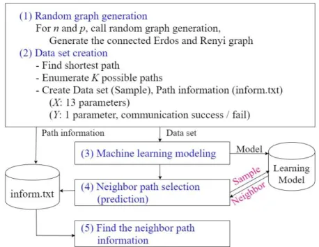
In this section, we describe our ML-NPS model depicted in Figure 1. ML-NPS model can be roughly categorized into the graph and data set creation and the machine learning modeling and prediction. Graph and data set creation part has two modules including the random graph generation (1) and the data set creation (2). Machine learning modeling and prediction part has three modules including the building of appropriate machine learning model (3), selection and prediction of the neighbor path (4), and the finding of the neighbor path information (5).
Figure 1. Machine learning based neighbor path selection (ML-NPS) model
We need a preparatory work including feature extraction for the neighbor path selection by using machine learning. Firstly, connected graph configuration is necessary. To generate the random graph, we use Erdos– Rényi (ER) model [11]. In the G (n, p) model, each edge is included in the graph with probability p independent from every other edge. Secondly, the shortest path from source to destination is necessary. We find it by using Dijkstra’s algorithm [12]. To use this shortest path as primary is reasonable in cost and time if there are no failures on the path. Therefore, we send data from source to destination using both the primary (the shortest) path and secondary (the neighbor) path simultaneously. Thirdly, data features to describe characteristics of the neighbor path selection problem are necessary. In the given network, we compute the distance between the two furthest nodes and set that as diameter. In addition, for selecting the neighbor path, we must compute the proximity factor and the sharing factor.
ML-NPS model enumerates K possible paths from source to destination and creates the data set used in the machine learning phase. ML-NPS model finds the optimal neighbor path with the maximum communication success probability using the machine learning. We generate random failures on the network including primary path and neighbor path by repeating iterations. We check whether the failures occur on the neighbor path. If
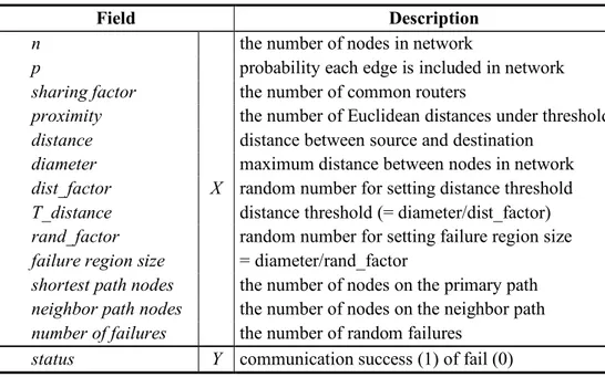
no failure occurs, communication is successful. From the above description, we can create the data set (Sample) including 13 input features (X) and one output parameter (Y) indicating the status of communication success or failure as like listed in Table 1.
Table 1. Data set for ML-NPS model
Field Description
n
X
the number of nodes in network
p probability each edge is included in network
sharing factor the number of common routers
proximity the number of Euclidean distances under threshold
distance distance between source and destination
diameter maximum distance between nodes in network
dist_factor random number for setting distance threshold
T_distance distance threshold (= diameter/dist_factor)
rand_factor random number for setting failure region size
failure region size = diameter/rand_factor
shortest path nodes the number of nodes on the primary path
neighbor path nodes the number of nodes on the neighbor path
number of failures the number of random failures
status Y communication success (1) of fail (0)
This data set is necessary only to train the machine learning model, so it does not include the detailed path information such as node indexes of the path. The detailed path information is saved on the inform.txt file. Later, we will obtain the information of best neighbor path in the finding module for the neighbor path information by searching the inform.txt file. Fields of inform.txt file is as followings: the node index of primary path, the node index of neighbor path, destination node, the node index of failure nodes, the number of node failures on the primary path, the number of node failures on the neighbor path, distance of primary path, and distance of neighbor path.
4. Performance evaluation
To implement the ML-NPS model, we code the whole modules in PYTHON 3.7 on Raspberry PI 4B (4GB RAM) computer. Both machine learning modeling module and neighbor selection (prediction) module use the Keras 2.2 as API and Tensorflow 1.13 as the machine learning library. For the performance evaluation of our model, we firstly explain the accuracy rate of the proposed machine learning model, and then compare the neighbor path by our ML-NPS model and the neighbor path by the related heuristics- PROX, SHA, and PROX-SHA in terms of the communication success rate and the communication success prediction probability.
We use deep multi-layer perception model [13]. Since the number of attributes except status (success or fail) in the data set of Table 1 is 13, the first dense (hidden) layer reads 13 neurons and outputs 64 neurons. The second dense layer reads 64 neurons and outputs 64 neurons. The third dense layer reads 64 neurons and outputs 32 neurons. Last dense layer reads 32 neurons and outputs one neuron (status). Because Relu function is easy to perform the backward propagation, we use it as the activation function. Since the output is either communication success (1) or fail (0), we use the sigmoid function. For the model compilation, we use the
Table 2 shows the accuracy rate of our machine learning model for (n=20, p=0.15) and (n=30, p=0.1) respectively. The coordinates of nodes are generated in the 2-dimensional coordinate plane between (-100, -100) and (100, 100). The possible number of neighbor paths (K) is set to 5,000. The number of iterations for the random failures (I) for each path is set to 100. dist_factor and rand_factor are varied from 1 to 3, respectively.
Table 2. Accuracy rate (%) of machine learning in the ML-NPS model (n=20, p=0.15) (n=30, p=0.1) rand_factor dist_factor 1 2 3 1 2 3 1 2 3 98.6 96.8 95.2 95.1 92.4 82.3 98.4 95.8 94.0 95.5 87.4 86.7 98.2 95.1 93.0 94.8 90.5 81.8
In Table 2, as the dist_factor and rand_factor increase, the accuracy rate of learning model decrease. If dist_factor and rand_factor become larger, the failure_region size becomes smaller. This causes to limit of a several different cases, thus learning effect might be declined. The effect of n is not large. The range of accuracy rate is between 81.8% and 98.6% depending on the dist_factor and rand_factor. Therefore, we can state that our deep multi-layer perception model achieves high accuracy rate.
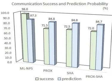
Figure 2 shows the communication success probability and prediction probability of ML-NPS, PROX, SHA and PROX-SHA when the number of possible paths (K) is 200 and the number of iterations for the random failures (I) for each path is 20. To simulate the geographically correlated failure, we set dist_factor and rand_factor to 5, respectively.
Mean communication success rates for (n=20, p=0.15) and (n=30, p=0.1) are 98.0% for ML-NPS, 71.5% for PROX, 72.5% for SHA, and 72.0% for PROX-SHA. Mean communication success prediction probabilities for (n=20, p=0.15) and (n=30, p=0.1) are 87.3% for ML-NPS, 84.8% for PROX, 84.8% for SHA, and 84.7% for PROX-SHA. On the communication success probability, the neighbor path by ML-NPS can transfer data from source to destination successfully more than the related heuristics by 26% on the average.
5. Conclusions
This paper has focused on the use of machine learning to the neighbor selection problem in case geographically correlated failures occur simultaneously on the communication network. For this purpose, we presented machine learning neighbor path selection (ML-NPS) model. We extracted data features describing the neighbor path selection problem well. Huge amount of data set was used for model training on tiny computer- Raspberry PI 4 computer. Accuracy rate of our model in the learning was between 81.8% and 98.6%. Based on comparing the communication success rate between the neighbor path obtained by our ML-NPS model and the existing neighbor path selection heuristics, the success rate of our model was 26% higher on average than the communication success rate of the existing heuristics. In this study, we dealt with only binary classification model covering the success and failure of the neighbor path. In the future, the development of multiple classification models including the success and failure of the primary path are expected.
References
[1] Z. Zhang and S. Chen, “Capacity-aware multicast algorithm on heterogeneous overlay networks,” IEEE Trans. Parallel Distribution System, Vol. 17, No. 2, pp. 135-147, 2006.
DOI: http://doi.org/10.1109/TPDS.2006.19
[2] N. Feamster, D. Anderson, H. Balakrishnan, and M. F. Kaasheok, “Measuring the effects of Internet path faults on reactive routing,” SIGMETRICS Performance Review, Vol. 31, No. 1, pp. 126-137, 2003.
DOI: http://doi.org/10.1145/885651.781043
[3] K. Kim and N.Venkatasubramanian, ”Assessing the impact of geographically correlated failures on overlay-based data dissemination,” in Proc. of IEEE Global Telecommunications Conference, Miami, USA, pp. 1-5, 2010. DOI: http://doi.org/10.1109/GLOCOM.2010.5685229
[4] Y. Lee, “Neighbor selection considering path latency in overlay network,” Journal of Natural Science, KNUE, Vol. 2, pp. 25-32, 2013.
[5] Y. Lee, “A path selection model considering path latency in the communication network with geographically correlated failures,” ICIC Express Letters, Vol. 13, No. 9, 2019.
DOI: http://doi.org/10.24507/icicel.13.09.789
[6] O. Simeone, “A very brief introduction to machine learning with applications to communication systems,” IEEE Trans. on Cognitive Communication and Networking, Vol. 4, No. 4, pp. 648-664, 2018.
DOI: http://doi.org/10.1109/tccn.2018.2881442
[7] T. Gruber, S. Cammerer, J. Hoydis, and S. Ten Brink, “On deep learning-based channel decoding,” in Proc. of 51st Annual Conference on Information Sciences and Systems(CISS), pp.1-6, 2017.
DOI: http://doi.org/10.1109/CISS.2017.7926071
[8] D. Deltesta, M. Danieletto, G. M. Di Nunzio, and M. Zorzi, “Estimating the number of receiving nodes in 802.11 networks via machine learning techniques,” in Proc. of IEEE Glob. Commun. Conference. (GLOBECOM), pp. 1-7, 2016.
DOI: http://doi.org/10.1109/GLOCOM.2016.7841821
[9] D. K.Bangotra, Y. Singh, and A. Selwal, “Machine learning in wireless sensor networks: challenges and opportunities,” in Proc. of Fifth Int. Conf. on Parallel, Distributed and Grid Computing(PDGC), pp. 534-539, 2018. DOI: http://doi.org/10.1109/PDGC.2018.8745845
[10] M. Chen,W.Saad,C. Yin, and M.Debbah,”Echo state networks for proactive caching in cloud-based radio access networks with mobile users,” IEEE Trans.Wireless Commun., Vol. 16, No. 6, pp. 3520-3535, 2017. DOI: http://doi.org/10.1109/TWC.2017.2683482
[11] Erdos and Renyl model, https://www.geeksforgeeks.org/erdos-renyl-model-generating-random-graphs/.
[12] E. W. Dijkstra, “A note on two problems in connection with graphs”, Numerishe Mathematik, Vol. 1, pp. 269-271, 1959.
DOI: http://doi.org/10.1007/BF01386390