A Polynomial Time Approximation Scheme for Enormous Euclidean Minimum Spanning Tree Problem

논문 2011-48CI-5-9

대형 유클리드 최소신장트리 문제해결을 위한 다항시간 근사 법

( A Polynomial Time Approximation Scheme for Enormous Euclidean Minimum Spanning Tree Problem )

김 인 범^**

( Inbum Kim

요 약

유클리드 최소 신장 트리(EMST) 문제는 2차원 평면상에 존재하는 입력노드들을 최소 비용으로 연결하는 것이다. EMST 와 같은 다항 시간문제에 대하여 연구된 알고리즘들은 수많은 입력들에 대하여 최적의 해를 얻기 위해 매우 많은 시간을 필요 로 한다. 본 논문에서는 이 문제에 대한 해를 구하기 위해 분할과 병렬기법을 활용한 다항 시간 근사법(PTAS)을 제안하는데, 이 기법은 비교적 짧은 시간 내에 매우 큰 근사 EMST를 생성할 수 있다. 순수 PTAS는 비-다항 시간문제를 위해 개발되었 지만, 다이내믹 프로그래밍을 활용하여 이것을 대형 EMST에 적용하였다. 제안된 방법에 의해 생성된 15,000개의 입력 단말 노드와 16개의 분할 영역으로 구성된 근사 EMST의 생성 실험에서, 직렬 방식은 89%, 병렬 방식은 99%의 실행시간의 감축을 보였다. 따라서 본 논문에서 제안하는 방법은 평면상의 매우 많은 수의 입력 단말 노드에 대하여 근사 EMST를 신속히 구축 해야 하는 응용에 잘 적용될 수 있다.

Abstract

The problem of Euclidean minimum spanning tree (EMST) is to connect given nodes in a plane with minimum cost.

There are many algorithms for the polynomial time problem as EMST. However, for numerous nodes, the algorithms consume an enormous amount of time to find an optimal solution. In this paper, an approximation scheme using a polynomial time approximation scheme (PTAS) algorithm with dividing and parallel processing for the problem is suggested. This scheme enables to construct a large, approximate EMST within a short duration. Although initially devised for the non-polynomial problem, we employ naïve PTAS to construct a vast EMST with dynamic programming.

In an experiment, the approximate EMST constructed by the proposed scheme with 15,000 input terminal nodes and 16 partition cells shows 89% and 99% saving in execution time for the serial processing and parallel processing methods, respectively. Therefore, our scheme can be applied to obtain an approximate EMST quickly for numerous input terminal nodes.

Keywords : Euclidean Minimum Spanning Tree; Polynomial Time Approximation Scheme; Portal

Ⅰ. Introduction

Minimum Spanning Tree(MST) is a minimum length tree connecting all terminal nodes with some given edges. Euclidean Minimum Spanning

* 정회원, 김포대학 IT학부

(School of Information Technology, Kimpo College) 접수일자: 2011년4월26일, 수정완료일: 2011년8월29일

Tree(EMST) is also a minimum length tree that connects all terminal nodes without given edges.

These trees can be used for network topology, routing, circuit design, and road construction.

Most published algorithms for them may encounter some difficulties in real-world special cases, for example, in dealing with many terminal nodes.

Another example of obstacles may be in an area

comprising some subareas that work independent of each other. Sometimes a node of one subarea seeks to communicate with nodes of other subareas. If the entire mechanism for locating and connecting terminal information is hidden or is unknown, management and communication within the system may encounter serious difficulties. For numerous decentralized terminal nodes processed independently, excessive execution time can be addressed via optimization of the MST. For partially independent subareas, a decentralized system can provide efficient solutions for the management of network security or hierarchy information gradation.

In this paper, our proposed scheme employs a Polynomial Time Approximation Scheme (PTAS) that has been devised to solve the Euclidean Travelling Salesman Problem (TSP), which is a NP problem

[1-3]. The scheme constructs a tree that connects

numerous terminal nodes that are located nearly evenly on a plane with minimum cost. By modifying PTASs devised for NP problems, our scheme can construct an approximately EMST in a short execution time. To justify our scheme, a huge EMST problem is selected and applied as a test case.

A particular merit of our scheme is its design facilitation through which the customer’s individual demands can be satisfied. Specifically, the target tree can be designed to focus on reduction of execution time or on a particular approach to optimize a MST.

Ⅱ. Background and Related Works

To connect

N

N-1

et al

N

E

pointer machine. The major difference between a EMST and a general MST is that the former does not have edges as input. That is, it connects all input vertices at a minimum cost. A simple methodology for this tree is to make complete connections for the given vertices and then to employ an efficient algorithm of general MST. The product of this method is an EMST.

Given

N

P

P

P

× log= ^{ ×}× log= ^× log when the number of edges of a Delaunay Triangular graph is made proportional to the number of vertices and applied to a general MST.

In a wireless sensor network, a MST can be used in the design of network topology and routing protocols. When designing a wireless sensor network system, energy efficiency of sensor nodes is a very important factor. To improve the energy efficiency of sensor nodes, J. Li

et al

Kim

et al

PTAS is a form of approximation algorithm for finding a solution with an allowable error ^{  } of the optimal solution. For example, for the Euclidean Traveling Salesman Problem (ETSP), PTAS can find a travel distance with ^{  } of additional moving distance from the shortest optimal travel. Arora showed that the ETSP can be solved in ^{} time by using PTAS for a ^{  } approximation of the TSP

optimal solution for N given nodes on plane^[1～2]. J.

Kim

et al

Ⅲ. Proposed Scheme

Our proposed scheme for an enormous EMST partially uses definitions and concepts reported in the literature ^[1,2,15]. The given problem area is divided by some rectangular forms. Sides of each rectangle are parallel or vertical against the axis of coordinates.

Size of a rectangle is defined as length of its long side. A target optimal tree is an optimal connecting structure, and a nonguaranteed optimal tree is defined as a connecting structure. Cost of a connecting structure is the sum of the edge lengths of the structure. The line separator of a rectangle

R

R

R

Divisions terminate when the size of the subrectangle reaches a determined value. Portals for parent rectangle are nodes located on the sides of the offspring rectangles. Portals are located between two ends of the rectangle sides. Length between two

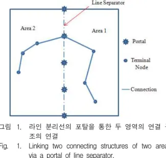
그림 1. 라인 분리선의 포탈을 통한 두 영역의 연결 구 조의 연결

Fig. 1. Linking two connecting structures of two areas via a portal of line separator.

adjacent two portals is the same in same layer, and number of portals yielded in every dividing layer is equal. Merging of two areas (rectangles) may occur on some portals to link two connecting structures of the areas.

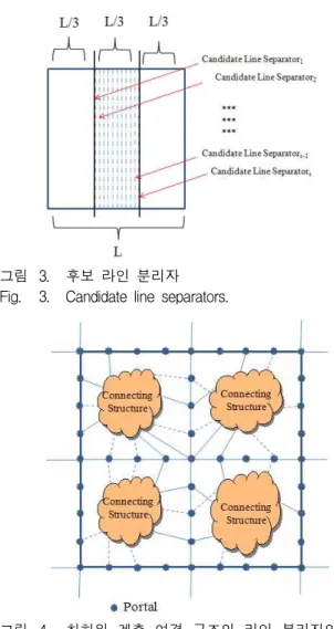
Fig. 1 shows the linking of a connecting structure of Area 1 to a connecting structure of Area 2 only on a portal of line separator when two problem areas are merged. For a structure that is closer to optimal, portals examined in the bottom layer should all be combinations of portals on all line separators. Among the combinations of each layer, some portals with the least costly final connecting structure that is built in the top layer are selected in each layer. Fig. 2 represents a problem area hierarchy that is partition-designed for applying PTAS to an enormous EMST. There are 16 partition cells in the bottom layer and 8 subareas in Layer 2 that are formed through merging two adjacent areas of the bottom layer. By the same method, a connecting structure in each area of the upper layer is built by merging two constructed structures in two adjacent areas of the under layer. In the top layer, all information on connecting structures built by every combination of all line separators and all portals in the lower layers can be acquired. Using that information, a minimum cost connecting structure is selected for an approximate MST. In Fig. 3, selecting a line separator is shown. A candidate line separator is a line parallel to the height of the rectangle problem

그림 2. 연결구조의 계층화

Fig. 2. Hierarchy for connecting structure.

그림 3. 후보 라인 분리자 Fig. 3. Candidate line separators.

그림 4. 최하위 계층 연결 구조의 라인 분리자의 포털 을 이용한 병합을 통해 생성 가능한 연결 구조 Fig. 4. Candidate merged connecting structure built with

bottom layer connecting structures through some portals on line separators.

그림 5. 트리 길이의 단축을 위한 후처리 작업 Fig. 5. Post processing for tree length curtailment.

area. Candidate line separators may locate on one of

 ∼  rectangle width

L

Step 1: For each candidate line separator, generate portals, respectively.

Step 2: For each partition cell of bottom layer, all connecting structures are built by brute-force method, respectively, with all combinations of portals generated in Step 1 and candidate line separators.

Step 3: For every combination of candidate line separators and portals, adjacent connecting structures of under layer are merged to form all connecting structures in next upper layer. Information for each connecting structure is saved in table entry.

Step 4: For next upper layer, repeat Step 3 for until all candidate connecting structures until top layer is built.

Step 5: In top layer, select minimum-cost connecting structure from all candidates using stored table entry information;

then investigate and collect all lower-layer connecting structures composed of selected connecting structure using table information.

Step 6: Perform post-process on final selected connecting structure to build final PTAS approximate Euclidean minimum spanning tree.

그림 6. PTAS를 이용한 대형 근사 최소 트리의 생성 알고리즘

Fig. 6. algorithm for constructing an enormous approximate Euclidean minimum spanning tree using PTAS.

each layer, lines with which minimum cost connecting structure can be built in the top layer become final line separators.

Fig. 4 represents an example of merging connecting structures of the bottom layer via portals.

Every merged connecting structure of each layer will be considered as a candidate for the top layer. Fig. 5 presents a post process. Instead of linking the left- and right-side connecting structures of the line separator via a portal, if two nodes attached to the portal directly link to each other, the total length of the tree will be shorter than the tree before the post process. Fig. 6 is an outline of our algorithm for building an approximate enormous EMST using PTAS. With the algorithm and four partition cells of the bottom layer, connecting structures for a final approximate EMST are shown in Fig. 7. Two hundred input terminal nodes appear in Fig. 7(a). Fig.

7(b) shows an optimal EMST yielded by modified Prim’s algorithm for input terminal nodes ^[4]. Fig. 7(c)

(a) 입력 단말노드

(a) Input terminal nodes (b) 최적 유클리드 최소신장트리 (b) Optimal EMST

(c) 결정된 최상위 연결 구조 (c) Determined connecting

structure in top layer

(d) 후처리 PTAS 근사 최소트리 (d) Post processed PTAS

approximate MST 그림 7. 제안된 기법에서 연결구조의 선택 및 처리 과

정

Fig. 7. Selections and post processes of connecting structures in proposed scheme.

illustrates a final determined connecting structure.

Fig. 7(d) demonstrates the final approximate EMST, which is a result of the post process that cuts the connections to selected portals and makes new connections between the terminal nodes that were previously linked to the portals.

Ⅳ. Experiment and Analysis

Experimental parameters for the proposed scheme are terminal node number and partition cell number of bottom layer. Results of the analysis are tree length approximation of constructed tree and execution time for tree construction. Approximate rate of length is determined by comparing the length of the tree constructed by our proposed scheme with the length of an optimal MST constructed by the modified Prim’s algorithm. In our experiments, a candidate line separator located on ^rectangle wide

(a) 입력 단말노드

(a) Input terminal nodes (b) 최적 유클리드 최소신장트리 (b) Optimal EMST

(c) 분할 영역 = 2

(c) Partition cell = 2 (d) 분할 영역 = 4 (d) Partition cell = 4

(e) 분할 영역 = 8

(e) Partition cell = 8 (f) 분할 영역 = 16 (f) Partition cell = 16 그림 8. 분할 영역 수의 변화에 따라 생성된 PTAS 근

사 최소 신장 트리(단말노드=3000, 라인 분리선 당 최대 포털 수=2)

Fig. 8. PTAS approximate minimum spanning trees constructed with different numbers of partition cell (terminal node = 3000, maximum portal number per line separator = 2).

L

Although it introduces some error in tree length, this simplification makes the proposed scheme easy to implement.

Numbers of randomly generated terminal nodes are 3000, 6000, 9000, 12000, and 15000. Each node has no

duplicate coordination in the plane and is located a little bit apart from the line separators of each layer.

Numbers of partition cells of the bottom layer are 2, 4, 8, and 16, and distribution of terminal nodes is nearly even. If partition cells are greater in number, terminal nodes that belong to each cell will be fewer, and handling them will be easier. If the number of partition cells of the bottom layer is smaller, the tree produced by our scheme will share more similar characteristics with an optimal MST, which can handle all terminal nodes.

In our experiments, we construct an optimal MST by modified Prim’s algorithm for comparison with the trees constructed by our proposed scheme. Our scheme was implemented by C++ and executed on a laptop with an Intel 1.83 GHz processor and 2 Giga byte of RAM.

Fig. 8(a) and Fig. 8(b) show 3000 randomly generated terminal nodes and an optimal EMST. For 3000 terminal nodes, Fig.s 8(c) to 8(f) show approximate EMSTs constructed by our scheme with different numbers of partition cells in the bottom layer. For numbers 2, 4, 8, and 16, the resulting trees can be seen in Fig.s 8(c), (d), (e), and (f), respectively. Dashed circles represent selected portals and their connections in the pictures.

1. Lengths and Overheads of the Trees

(a) 최적 트리와 PTAS 근사 트리간의 길이 (a) Lengths of optimal and PTAS approximate trees

(b) 최적트리와 PTAS 근사트리간의 길이오차 비율 (b) Error ratios between lengths of optimal and PTAS

approximate trees

그림 9. 단말노드의 수와 분할 영역의 변동에 따른 PTAS근사 최소 신장트리의 길이

Fig. 9. Lengths of PTAS approximate minimum spanning trees constructed with different numbers of terminal node and partition cells.

area. If the scheme can handle fewer terminal nodes in a larger number of partition cells, aggregated error of the constructed tree may be larger.

2. Effects of Post-Process

If triangle distance theorem applies to final connecting structures built by our proposed scheme, the new tree can be close to the optimal tree. When two nodes are indirectly connected via a portal in a final connecting structure in the top layer, if two

nodes connect directly to each other, the length of the new tree can be curtailed. When terminal nodes are distributed nearly evenly, if the number of terminal nodes is smaller, the effect of post process may be greater. Further, although the number of terminal nodes is larger, if the whole problem area is larger, the effect of post process may be also greater.

Fig. 10 shows that if the number of terminal nodes is smaller, the effect of post process is more pronounced. When the partition cell number is four, if the number of terminal nodes is 3000, the saving length is 0.34 and the saving ratio is 0.08%; if the number of terminal nodes is 15000, the saving length is 0.18 and the saving ratio is 0.02%.

(a) 후처리 작업 후의 절감된 트리 길이 (a) Curtailment of tree lengths after post process

(b) 후 처리 작업 후의 길이 절감 비율 (b) Length curtailment ratio after post process 그림 10. 후 처리 결과

Fig. 10. Results of post process.

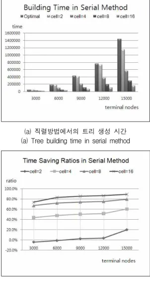
3. Times for Tree Construction through the Serial Method

Fig. 11 shows execution times of PTAS approximate MST constructed by the serial method with given experimental parameters. In the serial method, among areas in a layer only one is processed at a time according to a predefined order and then the next one is processed. Fig. 11 shows that the more partition cells present in the bottom layer, the greater is the saving ratio of execution time. When the terminal node number is 15000, the time saving ratio of the tree constructed with sixteen partition cells is 89.2%, and the ratio of the tree constructed

(a) 직렬방법에서의 트리 생성 시간 (a) Tree building time in serial method

(b) 직렬방법의 시간 절감 비율 (b) Time curtailment ratio by serial method 그림 11. 직렬 PTAS 근사 최소 신장트리 생성 시간 Fig. 11. Construction time of PTAS approximate minimum

spanning tree by the serial method.

with two partition cells is 20.1%. If the number of terminal nodes is more for the same number of partition cells, then the time saving ratios are even somewhat higher. When the partition cell number is sixteen, the PTAS approximate MST constructed by the serial method with 3000 terminal nodes shows a 73.7% time saving ratio compared to the optimal tree, and the PTAS tree with 15000 terminal nodes achieves a savings ratio of 89.2%.

Thus, we have demonstrated via laboratory experiments that our scheme, which does not require an optimal MST, deals successfully with a very large number of terminal nodes and also does not take too much time for building the application, so it can be a good practical choice.

4. Times for Tree Construction through the Parallel Method

Fig. 12 shows execution times for constructing PTAS approximate MSTs by the parallel method with given experimental parameters. In the parallel method, each partition cell of the bottom layer may have its own processor working independently on its connecting structures. Because execution time for the bottom layer is the longest of all execution times for constructing a tree, connecting structures of other layers except for the bottom layer can be built by similar application of the serial method. Through experimental analysis, we have verified that most of the execution time is spent in making connecting structures for the bottom layer. Therefore, if each step for the bottom layer is processed in parallel, much time can be saved. However, if there are many merging steps to construct the target tree, more time savings can be expected by using some well-placed processors. Fig. 12 shows that when the number of partition cells is the same, if the number of terminal nodes increases, savings ratios of execution time for constructing trees either increase somewhat or show no change, as with the serial method. When the number of terminal nodes is the same, if the partition cells of bottom line are greater, the execution time is

(a) 병렬방법에서의 트리 생성 시간 (a) Tree building times in parallel method

(b) 병렬방법의 시간 절감 비율 (b) Time curtailment ratio by parallel method 그림 12. 병렬 PTAS 근사 최소 신장트리 생성 시간 Fig. 12. Construction time of PTAS approximate

minimum spanning tree by the parallel method.

much shorter. Saving ratios for the parallel method are far greater than those for the serial method with regard to tree construction time.

Construction time using the parallel method for the PTAS approximate MST with 15000 terminal nodes and sixteen partition cells is 99% shorter than that for the optimal MST. This construction time is also 92.4% shorter than that for the PTAS tree using the serial method. Execution time using the parallel method for the PTAS tree with 15000 terminal nodes and two partition cells is 58% shorter than execution time for the optimal tree and 47.7% shorter than execution time using the serial method.

Therefore in an environment where use of the parallel method is possible, if each partition cell in the bottom layer is designed to be handled by its own processor, construction time for goal tree by our proposed parallel method can be much less than that using the MST algorithm and also less than that using the serial method described in section 4.3 above.

5. Running Time

Running time for constructing a MST by Prim’s algorithm is ^× log. In the naïve algorithm for the EMST, it is ^^× log ^, because

^ time is needed for creating complete connections. Running time for the approximate EMST proposed in this paper using PTAS is composed of time for building connecting structures of each partition cell in the bottom layer, time for making table entries for connecting structures in each layer, and time for table retrievals. Time for building connecting structures of each partition cell of the bottom layer is as follows:

In serial method:





 ×  × _× _^

(1)

In parallel method:

max_{ ≤  ≤ }  ×  × _× _^

(2)

In Expressions (1) and (2),

l

k

n

represents the number of terminal nodes that belong to partition cell

i

n

N

k

n

t

is the time per each terminal node for building a connecting structure for the MST. The symbol

m



  



_ where

r

PTAS is designed by

l

m

In the serial method:





 ×  × _× _^×



  



_^^

(3)

In the parallel method:

max_{ ≤  ≤ }  × ×_× _^  × max_{ ≤  ≤ } _^  ^

(4)

E

E





  



^     

(5)

In expression (5),

d

d

^  _× _×^ ≤^

(6)

t

t

Ⅴ. Conclusions

It should be noted that our proposed scheme is encumbered with many restrictions. Processing steps of the scheme are simplified by some methods such

as the cut-branch technique. These restrictions may affect the approximation rate of the trees that we construct. However, if original PTASs without restrictions are applied to a problem, huge execution times and memories will be required, which will throw into doubt the practical usage of our scheme.

We have also attempted to use our proposed scheme to solve other problems that have been solved by well-known algorithms but which in special case of real world, can issue some practical difficulties. Through our scheme, running time and memory space are expected to be saved for the problems. Another work is to study the proposed PTAS under diverse environments. Applying our scheme to non-even distributed terminal nodes is an example. In this paper, we assumed nearly even distributed terminal nodes. In real world application, a solution of PTAS for non-even distributed terminals may be necessary.

References

[1] S. Arora, “Polynomial Time Approximation Schemes for Euclidean TSP and Other Geometric Problems,” Journal of ACM, Vol.45, no.5, pp.753-782, 1998.

[2] S. Arora, “Nearly Linear Time Approximation Schemes for Euclidean TSP and Other Geometric Problems,” in Proc. of the 38th IEEE Symposium on Foundations of Computer Science 1997, Miami, pp.554-563, 1997.

[3] X. Cheng, J. Kim and B. Lu, “A Polynomial Time Approximation Scheme for the Problem of Interconnecting Highways,” Journal of Combinatorial Optimization, Vol.5, no.3, pp.327-343, 2001.

[4] T.H. Cormen, C.E. Leiserson, R.L. Rivest and C.

Stein, Introduction to Algorithm, 2nd ed., MIT Press, Cambridge, pp.525-579, 2001.

[5] S. Pettie and V. Ramachandran, “An Optimal Minimum Spanning Tree Algorithm,” Journal of the ACM, Vol.49, no.1, pp.16-34, 2002.

[6] F.P. Preparata and M.I. Shamos, “Computational Geometry: An Introduction,” Springer, New York, 1985.

[7] J. Li, D. Cordes and J. Zhang, “Power-Aware

Routing Protocols in Ad Hoc Wireless Sensor Networks,” IEEE Wireless Communications, Vol.12, no.6, pp.69-81, 2005.

[8] J. Kim and E. Goo, “Sharing Error Allowances for the Analysis of Approximation Schemes,”

Journal of the Institute of Electronics Engineers of Korea TC, Vol.46, no.5, pp.1-7, 2009.

[9] J. Kim, M. Cardei, I. Cardei and X. Jia, “A Polynomial Time Approximation Scheme for the Grade of Services Steiner Minimum Tree Problem,” Journal of Global Optimization, Vol.24, pp.437-448 , 2002.

저 자 소 개

김 인 범

대한전자공학회논문지

TC편 47권 11호 2010년 11월, 7-13쪽 참고