Selection of Optimal Values in Spatial Estimation of Environmental Variables using Geostatistical Simulation and Loss Functions

(1)

Jour. Korean Earth Science Society, v. 31, no. 5, p. 437−447, September 2010

Selection of Optimal Values in Spatial Estimation of Environmental Variables using Geostatistical Simulation and Loss Functions

No-Wook Park*

Department of Geoinformatic Engineering, Inha University, Incheon 402-751, Korea

Abstract: Spatial estimation of environmental variables has been regarded as an important preliminary procedure for decision-making. A minimum variance criterion, which has often been adopted in traditional kriging algorithms, does not always guarantee the optimal estimates for subsequent decision-making processes. In this paper, a geostatistical framework is illustrated that consists of uncertainty modeling via stochastic simulation and risk modeling based on loss functions for the selection of optimal estimates. Loss functions that quantify the impact of choosing any estimate different from the unknown true value are linked to geostatistical simulation. A hybrid loss function is especially presented to account for the different impact of over- and underestimation of different land-use types. The loss function-specific estimates that minimize the expected loss are chosen as optimal estimates. The applicability of the geostatistical framework is demonstrated and discussed through a case study of copper mapping.

Keywords: loss function, risk, simulation, expected loss, spatial estimation

Introduction

Environmental variables such as heavy metal or particulate matter (PM) concentrations are usually collected at a limited number of locations. In general, further analysis requires attribute values at all locations in the study area of interest. Thus, spatial estimation or interpolation is required to obtain exhaustive attribute values (Cho and Jeong, 2009;

Park, 2009). A lot of interpolation algorithms have been developed and applied to geoscientific tasks where spatial data are dealt with. Nowadays multivariate kriging has often been applied to integrate multiple data for the improvement of prediction accuracy (Kwon and Oh, 2002; Oh, 2005; Park et al., 2009).

Although spatial estimation of environmental variables is an important procedure, the generation of maps is not a final goal but a preliminary procedure for further analysis. A spatial distribution map of environmental variables is generally used as basic information for making a decision, e.g., remediation of contaminated areas by heavy metal or ecological

impact assessment. The map generated by any interpolation algorithms, however, inevitably includes uncertainty associated with the estimation at unsampled locations. Thus, most decisions have to be made in the presence of uncertainty. Prior to any decisions, it is required to assess estimation uncertainty which should be reflected into subsequent decision-making processes (Morgan and Henrion, 1990).

Interpolation algorithms commonly used in Geographical Information System (GIS) or geoscience, e.g., inverse distance weighting, do not provide any quantitative measures of uncertainty. While geostatistical kriging including univariate and/or multivariate approaches provides both estimation values and error variance at unsampled locations. However, kriging variance is independent of data values but depends only on the data configuration (Goovaerts, 1997).

Hence, it cannot be regarded as a measure of uncertainty.

Besides traditional kriging algorithms such as ordinary kriging, geostatistics provides a probabilistic framework in which one can quantify uncertainty (Goovaerts, 1997; Deutsch and Journel, 1998; Chilès and Delfiner, 1999). In geostatistics, the uncertainty is usually modeled as a conditional cumulative distribution function (CCDF), which gives the probability that the

(해 설)

*Corresponding author: [email protected]

*Tel: 82-32-860-7607

*Fax: 82-32-863-1506

(2)

unknown random variable is no greater than any given threshold for continuous data (Goovaerts, 2001). For local uncertainty modeling, multi-Gaussian kriging or indicator kriging can be applied as a parametric or non-parametric approach, respectively. Since the early 1990s, stochastic simulation has been developed for spatial uncertainty modeling, and a lot of simulation algorithms such as sequential simulation, p-field simulation, and simulated annealing have been proposed and applied. Stochastic simulation generates a set of equi-probable realizations for unknown truth without smoothing effects. This set can be used to model the uncertainty by considering differences among realizations (Goovaerts, 1997; Deutsch and Journel, 1998). Due to this advantage, stochastic simulation has been preferred over kriging in uncertainty modeling.

As any decisions are made by using one unique value, in most cases, it is not common for decision- makers to use probability directly in the final decision- making stage (Leuangthong et al., 2008). Kriging- based estimates generated under a minimum variance criterion may not be appropriate for the task aiming to find large values such as pollutant contamination, because kriging typically smoothes out local details, small values tend to be overestimated, while large values are underestimated. Thus, an optimal and single value at unsampled locations should be chosen from uncertainty models constructed (i.e. CCDF model), regardless of type of algorithms used for uncertainty modeling. There are a lot of summary statistics that can be used as the best estimate such as mean or median of the CCDF. A common way to find the estimate is to compute mean values, also known as E- type estimates (Goovaerts, 1997). For kriging-based uncertainty models, conditional means are computed from the CCDF. In stochastic simulation, mean values are computed from the set of realizations. However, these values may not be optimal, because they are heavily dependent on the decision of interest.

Decisions based on incomplete knowledge or in the presence of uncertainty may incur loss. For example, let us suppose a toxic waste clean up task. The

uncertainty arises when the extent of contamination is estimated. If the estimates are too high, the cost associated with the remediation action should be too expensive due to an excessive cleaning (e.g., more than needed). On the other hand, underestimation may otherwise result in potential health problems. Thus, it is necessary to compute the optimal value that minimizes future loss or consequences due to a wrong decision making.

To quantify the penalty of loss resulted from the wrong decision, a loss function can be applied to the choice of the optimal value. The loss function quantifies the impact or loss associated with any estimate different from the unknown truth (Srivatava, 1987; Da Cruz, 2000; Leuangthong et al., 2008). This concept has been widely applied to mining or petroleum in geoscience (Da Cruz, 2000; Godoy et al., 2001; Deutsch, 2002). Despite its great potential in environmental thematic mapping, to our knowledge, main concepts and an example of soil data related to heavy metal contamination are only addressed by Goovaerts (1997, p. 340-346). Research on the application of loss functions linked to geostatistical simulation has not been carried out for spatial estimation of environmental variables.

This paper aims to illustrate how a loss function can be used in conjunction with geostatistical simulation to obtain the optimal estimate of environmental variables for improved decision-making. First, a set of alternative realizations for environmental variables is generated via stochastic simulation. Then, a loss function is defined to quantify the loss of over- and underestimation for variables of interest. As a main part of this study, a hybrid loss function, which accounts for the different penalty with respect to various land-use types, is presented and applied. The expected loss is computed by applying the loss function to each realization, and the estimate with the minimum expected loss is chosen as an optimal estimate. A case study of copper mapping in the Ogdong area, Korea is described to demonstrate the proposed scheme, as shown in Fig. 1.

(3)

Selection of Optimal Values in Spatial Estimation of Environmental Variables using Geostatistical Simulation and Loss Functions

439

Theory

Stochastic simulation

Unlike kriging that aims to find the best estimates in the least-squares sense, stochastic simulation focuses on generating a set of alternative realizations, which honor sample data values, and also reproduce statistics (e.g. histogram) and spatial structure (e.g.

variogram) of sample data without smoothing effects (Journel, 1996; Goovaerts, 1997). It can also be easily applied to change of support problems such as upscaling to the regular or irregular blocks in a non- parametric way. In addition, the set of alternative realizations can be used as input for any physical models in order to assess the impact of input uncertainty on response values.

Among several simulation algorithms reported in geostatistics literature, sequential indicator simulation is adopted in this study. Unlike sequential Gaussian simulation which assumes that data of interest should follow the multi-Gaussian distribution model, sequential indicator simulation does not require any Gaussian

hypothesis, and can be applied to any data sets with arbitrary distributions. Although this indicator approach is more time-consuming as the number of thresholding values increases, it is well suited for the highly-skewed data set such as geochemical data sets (Park, 2009).

The main concept of sequential simulation is that conditioning is extended to include all data available within a neighborhood of the interpolation grid, including the original sample data and all previously simulated values (Deutsch and Journel, 1998, p. 125).

Details on sequential simulation can be found in Goovaerts (1997) and Deutsch and Journel (1998).

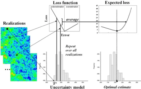
Before applying sequential indicator simulation, a local uncertainty model should be first constructed via indicator kriging. Within the indicator framework, sample data are first indicator-transformed into a set of K indicator values corresponding to K threshold values (Journel, 1983). Then, a random path visiting only once each interpolation node to be simulated is defined. At each interpolation node, the following 5 steps will be implemented until all interpolation nodes Fig. 1. Work flow adopted in this study for selecting an optimal value in a geostatistical context.

(4)

are visited (Goovaerts, 1997, p. 395):

1. K CCDF values are estimated by kriging with indicator transforms of neighboring original sample data and previously simulated values.

2. Any order relation deviations are corrected, and the complete CCDF is constructed by interpolation and extrapolation of these estimated probabilities.

3. A simulated value is drawn from that CCDF using a random number between 0 and 1 (i.e.

Monte-Carlo simulation).

4. This simulated value is added to the conditioning data set for all subsequent drawings.

5. The interpolation node is moved along the random path, and repeat steps 1 to 4.

The resulting set of simulated values represents one realization of the random function. Any number L of such realization can be generated by repeating L times the entire sequential process with different paths (Deutsch and Journel, 1998).

Loss function

A loss function is a penalty function that quantifies the consequence of choosing an estimate different from the unknown truth (Srivatava, 1987; Da Cruz, 2000; Leuangthong et al., 2008). As discussed in Srivastava (1987), the loss function depends on what

the estimate is being used for, not on what is estimated. That is, it depends on the uncertainty and the impact of a mistake or an incorrect decision.

The loss function takes various functional forms (e.g. linear or quadratic) to measure the penalty to both over- and underestimation (Morgan and Henrion, 1990). If a symmetric loss function is used, the penalty to overestimation is the same as that to underestimation. If the consequences of over- and underestimation are quite different, an asymmetric loss function should be used to reflect the different penalty.

Once the appropriate loss function has been specified, an optimal estimate should be such that the loss associated with the difference between the estimate and the true value is minimized. However, the determination of the actual loss requires the actual true value that is unknown in practice. Since the uncertainty about the true value can be modeled by the CCDF from kriging or by stochastic simulation, an alternative is to minimize the expected value of loss under the uncertainty model. That is, the optimal estimate is one that minimizes the expected loss (Srivastava, 1987; Goovaerts, 1997).

To compute the expected loss, uncertainty models and a loss function should be specified. In case of stochastic simulation, the uncertainty model can be

Fig 2. A procedure for finding an optimal estimate from the expected loss computed from simulated realizations and the loss function.

(5)

441

derived from the histogram of simulated values. Thus, the calculation of the expected loss is based on taking each realization value from stochastic simulation. First, one assumes that one realization (z*) is true and all of the others (zl) are estimates. Then, the estimation error given the true value and the loss attached to the estimation error are calculated, and the expected loss given the true value is derived using equation (1).

(1)

where N is the number of realizations and L(·) is a predefined loss function.

Above calculation steps are repeated for all possible true values (i.e. all realizations). The estimate returning the minimum loss is the best or optimal estimate. This procedure is illustrated in Fig. 2.

The determination of the optimal estimate depends on the shape of the predefined loss function. For some particular loss functions, the optimal estimates are available without any numerical computation (Morgan and Henrion, 1990; Goovaerts, 1997). Fore example, if a symmetric quadratic function is used as the loss function, the optimal estimate is the expected value of the CCDF or the mean value of realizations. The median estimate is the optimal one in case of the symmetric linear loss function of the absolute value of the estimation error. An asymmetric linear loss function returns the p-quantile of the CCDF as the

optimal value (Da Cruz, 2000).

Case Study

Study area and data

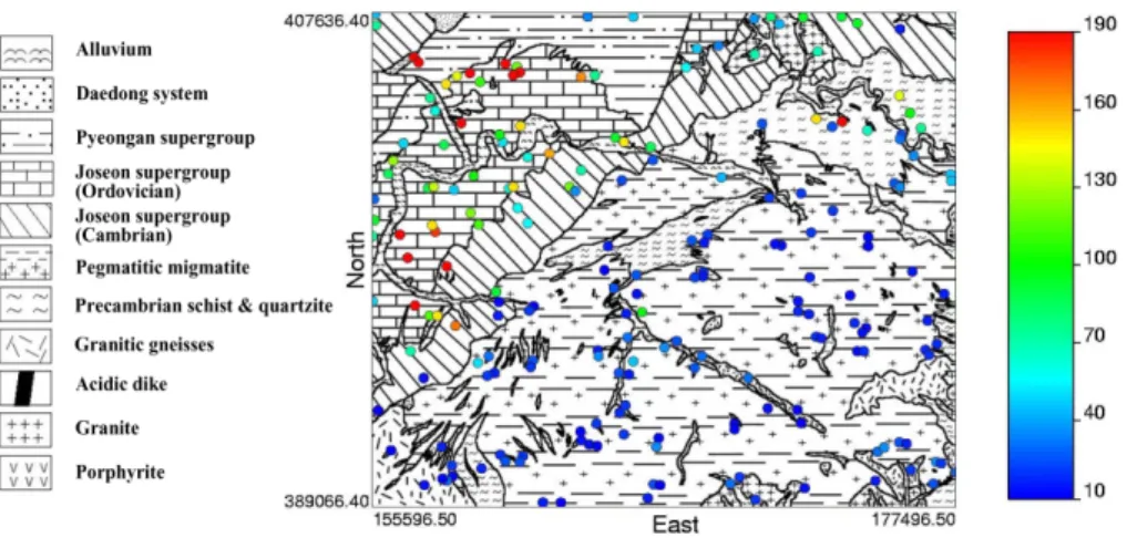
A case study of Ogdong, Korea was carried out to exemplify the usefulness of geostatistical simulation in conjunction with loss functions. Among various geochemical elements acquired from stream sediments at 198 locations (Lee et al., 1984), a copper element was experimentally chosen for the case study (Fig. 3).

Stream sediments were collected from the first-order streams with an average sampling density of one sample per 2 square kilometers (Lee et al., 1984).

Geologically, the study area comprises Precambrian metasediments, pegmatitic migmatite, the Cambrio- Ordovician Joseon Supergroup, the Late Carboniferous to Triassic Pyongan Supergroup, Jurassic (unnamed formation) and igneous rocks, such as granites, porphyritic intrusives, and dikes (Lee, 1966). The major part of the study area is composed of metasediments.

Generation of alternative realizations

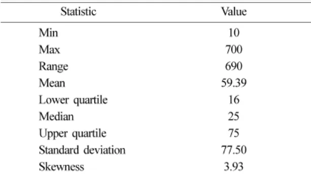
Prior to geostatistical analysis, basic statistical information was first extracted (Table 1). From descriptive statistics, it is observed that copper data are positively skewed with the skewness value of 3.93, and do not follow the Gaussian distribution.

E L z∗{ ( )} 1N---- L z∗ z( – l)

l 1=

∑

N

=

Fig. 3. Locations of copper sample data with the geological map. Symbols for sample locations are enlarged for visibility.

(6)

Thus, an indicator framework as a non-parametric approach is appropriate to this data, and sequential indicator simulation was applied to generate the set of alternative realizations. Nine thresholding values corresponding to nine percentiles of the sample

histogram were applied for indicator-transform of sample data. After indicator coding, nine experimental variograms were computed and modeled. Then, sequential indicator simulation was applied to generate 100 realizations. The whole geostatistical analysis was implemented by using GSLIB (Deutsch and Journel, 1998) and FORTRAN programming.

Two realizations among 100 realizations are shown in Fig. 4. The differences among 100 realizations provide a measure of uncertainty about the spatial distribution of copper values. Fig. 4c is a cumulative distribution of 100 simulated values at one grid point, which can be regarded as the CCDF at this point.

Defining loss functions

Once simulated realizations have been generated Table 1. Descriptive statistics of copper sample data

Statistic Value

Min 10

Max 700

Range 690

Mean 59.39

Lower quartile 16

Median 25

Upper quartile 75

Standard deviation 77.50

Skewness 3.93

Fig. 4. (a) 10^th realization, (b) 50^th realization, (c) a cumulative distribution of 100 realizations at one grid point.

(7)

443

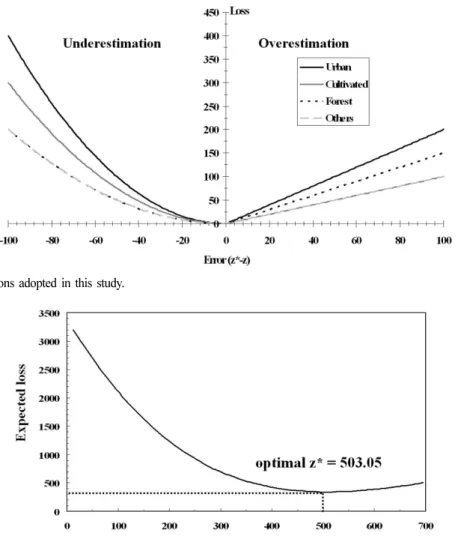
and the uncertainty has been modeled, the next step is to define a reasonable loss function. In this paper, a hybrid and asymmetric loss function is defined to reflect the different impact of various land-use types as well as that of over- and underestimation. If a symmetric loss function is chosen, the loss due to underestimation is the same as that due to overestimation. In many cases, however, this symmetric loss may not be appropriate. For example, in case of remediation tasks, the underestimation of contamination values may cause severe health problems than the unnecessary cost loss due to overestimation. In this case, an asymmetric loss function, which penalizes underestimation more than overestimation, is preferred. In addition, the impact of the estimation error may also vary according to the land-use types. For example, underestimation of contamination values may be more serious in urban or cultivated areas than in forest or other areas, due to more damage to human and crops. While, remediation as a consequence of overestimation may require more cost in forest due to more clear cutting efforts than in cultivated areas.

To account for above different impacts of over- and underestimation for land-use types, the hybrid asymmetric loss functions that are specific to land-use types are adopted. One criterion adopted is that a greater penalty should be given for the large underestimates due to more risk associated with

human health problems in major land-use types. Thus, quadratic and linear functions are applied for underestimation and overestimation, respectively. By using the quadratic function for underestimation, the small underestimates do not have great loss. As the underestimation errors increase, while, the loss increases rapidly and outweighs the loss of overestimation. Different weighting factors are considered to account for the different impact of the particular land-use type. In the quadratic function for underestimation, the greater weighting factor was multiplied for urban and cultivated areas than for forest, due to the greater risk associated with contamination of those land-use areas. The losses due to underestimation in urban and cultivated areas are 2 and 1.5 times, respectively, greater than the loss in forest. For overestimation, the greatest weighting factor was multiplied to the linear function in urban area. Unlike the case of underestimation, the loss function due to overestimation in forest is linear with the loss 1.5 times greater than the loss in cultivated areas, due to the fact that it is more expensive to clean forest areas than the more accessible cultivated areas. The absolute magnitude of the weighting factors was adjusted by considering the range of sample data and relative difference between under- and overestimation. These loss functions that are specific to both over/underestimation and laud-use types are summarized in equation (2) and Fig. 5.

(2)

Estimation results

For a series of possible estimates from 100 realizations, the expected loss in equation (1) was calculated. A digital land-use map provided by the Environmental Geographic Information System was

used to apply the loss functions that depend on the land-use types. By plotting the expected loss against the possible estimates, one can find the optimal estimate that minimizes the expected loss. Fig. 6 is one example of the expected loss curve computed at L z∗ z( – )

0.04 z∗ z⋅( – )² in urban

0.03 z∗ z⋅( – )² in cultivated if z∗ z≤ (underestimation) 0.02 z∗ z⋅( – )² in forest and others

2 z∗ z⋅( – ) in urban z∗ z–

( ) in cultivated and others if z∗ z> (overestimation) 1.5 z∗ z⋅( – ) in forest

⎩⎪

⎪⎪

⎪⎨

⎪⎪

⎧

=

(8)

one grid point whose CCDF is shown in Fig. 4c. At this point, the optimal value is 503.05 ppm, which returns the minimum expected loss.

The optimal estimates at all locations in the study area are shown in Fig. 7a. For the comparison purpose, ordinary kriging and the E-type estimates from 100 realizations are also computed and shown in Fig. 7b and 7c. Overall, large concentrations of cupper are observed in the west and north-western parts of the study area. These areas geologically correspond to Joseon and Pyeongan Supergroups. However, distinct relationships between geological boundary and spatial distribution of copper were not observed. As expected, the ordinary kriging estimates in Fig. 7b showed

smoothing effects. Large concentrations were underestimated and high-valued areas are very small due to the minimum variance criterion, compared with the optimal estimates. Unlike ordinary kriging, the E- type estimates in Fig. 7c tend to show less smoothing effects, although the average operator was applied.

The optimal estimates based on loss functions also show the local details of spatial variability of copper concentration. Due to the greater penalty for underestimation, the optimal value would be chosen toward near the higher quantile value, unlike the mean value of the distribution like the E-type estimates.

Thus, large values in western and north-western parts of the study area are distributed more broadly than the Fig. 5. Loss functions adopted in this study.

Fig. 6. Expected loss curve and optimal estimate indicated by the dashed line computed from the 100 simulated estimates at one grid point.

(9)

445

E-type estimates. For example, the optimal value of 503.05 ppm in Fig. 6 corresponds to the 0.76 quantile value of the CCDF shown in Fig. 4c. The major difference between the optimal and the E-type estimates is that the optimal estimates based on loss functions can account for different patterns in major land-use types. For additional information on interpretations, standard deviation values were computed from 100 realizations (Fig. 4d) and compared with the spatial estimation results. High- valued areas in all estimation results showed large standard deviation values. That means that greater uncertainty is attached to the estimation of large values. When such uncertainties exist and can not also be negligible, the estimate computed by the presented scheme is optimal under the loss functions based on

different penalty to over- and underestimation, unlike kriging or E-type estimates that are optimal only to the minimum variance or equal penalty criterion, respectively. It should be noted that this optimal estimate is best given both the uncertainty model and the loss functions. If different loss functions are employed, thus, the optimal estimate would be changed.

Discussion and Conclusion

Traditional estimation of environmental variable has been based on the application of any interpolation algorithms to obtain one single value at unsampled locations. Although decisions are typically based on this one estimation value, however, this kind of Fig. 7. Estimation results; (a) optimal estimates based on loss functions, (b) ordinary kriging, (c) E-type estimates of 100 realizations, (d) standard deviation of 100 realizations.

(10)

deterministic value may not be appropriate to be used for further decision-making due to uncertainty attached to this estimation procedure. Thus, it is necessary to consider this uncertainty to find optimal estimation values. Traditional kriging estimates are only optimal under the minimum variance criterion. If the objective of problems is changed, a certain criterion for finding best estimates may not be optimal.

In relation to the selection of optimal estimates, a geostatistical framework is illustrated that can quantify the uncertainty through stochastic simulation, and incorporate the concept of loss functions in order to account for the consequences of choosing wrong decisions. Especially, the application of loss functions can be regarded as a general approach in decision- making applications by considering both uncertainty and risk. Loss functions can reflect different impact of making a mistake in a flexible way by different definitions in the problem at hand. The usual least- squares criterion, which is often adopted in kriging or E-type estimation, can be expressed by the loss function that penalizes equally over- and underestimation.

Main contribution of this paper lies in the formulation of loss functions that can account for the different impacts of over- and underestimation for various land- use types. The concept and applicability of loss functions in conjunction with geostatistical simulation were demonstrated through a case study of copper mapping. The case study results indicated that this approach could consider the uncertainty of the copper concentrations, and determine the optimal estimates that can depict local details of copper concentrations unlike ordinary kriging. These loss function-specific optimal estimates would be used for further decision- making, e.g. classifying the study area as contaminated or safe. For the presented scheme to be more applicable, proper validation based on independent samples should also be implemented. Large uncertainty in high-valued areas observed in this case study may be reduced and proper interpretations may be done by considering geological and topographical effects during the generation of simulated realizations.

Sequential simulation with local means would be

applicable to this purpose.

Although it leaves the critical job of the choice of loss functions, this approach can also be extended to various decision-making problems under uncertainty, provided that both modeling uncertainty by geostatistics experts and defining loss functions by practitioners are properly or reasonably designed. For example, improved geostatistical inversion of geophysical parameters (Oh, 2008), and the value of information analysis both for acquiring additional sampling data (Solow and Ratick, 1994) and for choosing the best data set (De Bruin et al., 2001) would be promising fields of application.

Acknowledgment

This work was supported by INHA UNIVERSITY Research Grant.

References

Chilès, J.-P. and Delfiner, P., 1999, Geostatistics: Model- ling Spatial Uncertainty. Wiley, NY, USA, 695 p.

Cho, H.-L. and Jeong, J.-C., 2009, The distribution analysis of PM10 in Seoul using spatial interpolation meth- ods. Journal of the Korean Society of Environmental Impact Assessment, 18, 31-39. (in Korean)

Da Cruz, P.S., 2000, Reservoir management decision-making in the presence of geological uncertainty. Ph.D. the- sis, Stanford University, Stanford, USA, 221 p.

De Bruin, S., Bregt, A., and Van De Ven, M., 2001, Assessing fitness for use: the expected value of spatial data sets. International Journal of Geographical Informa- tion Science, 15, 457-471.

Deutsch, C.V., 2002, Geostatistical Reservoir Modeling.

Oxford University Press, NY, USA, 376 p.

Deutsch, C.V. and Journel, A.G., 1998, GSLIB: Geostatisti- cal Software Library and User's Guide. 2nd ed., Oxford University Press, NY, USA, 369 p.

Godoy, M.C., Dimitrakopoulos, R., and Costa, J.F., 2001, Economic functions and geostatistical simulation applied to grade control. In Edwards, A.C. (ed.), Mineral Resources and Ore Reserve–The AusIMM Guide to Good Practice. The Australasian Institute of Mining and Metallurgy, Melbourne, Australia, 591-599.

Goovaerts, P., 1997, Geostatistics for Natural Resources Evaluation. Oxford University Press, NY, USA, 483 p.

Goovaerts, P., 2001, Geostatistical modeling of uncertainty

(11)

447

in soil science. Geoderma, 103, 3-26.

Journel, A.G., 1983, Non-parametric estimation of spatial distributions. Mathematical Geology, 15, 445-468.

Journel, A.G., 1996, Modeling uncertainty and spatial dependence: stochastic imaging. International Journal of Geographical Information Science, 10, 517-522.

Kwon, B.-D. and Oh, S.-H., 2002, Bayesian inversion of gravity and resistivity data: detection of lava tunnel.

Journal of the Korean Earth Science Society, 23, 15-29.

Lee, D.-S., 1966, Explanatory Text of the Geological Map of Ogdong Sheet. Geological Survey of Korea, Seoul, Korea, 30 p.

Lee, J.-S., Hong, Y.-K., Kim, S.-Y., Yun, H.-S., Jin, M.-S., and Lee, C.-Y., 1984, Geochemical Maps for Ogdong Sheet in the Taebagsan Mineralized Belt. Korea Insti- tute of Energy and Resources, Daejeon, Korea, 35 p.

Leuangthong, O., Khan, K.D., and Deutsch, C.V., 2008, Solved Problems in Geostatistics. Wiley, NJ, USA, 207 p.

Morgan, M.G. and Henrion, M., 1990, Uncertainty: A Guide to Dealing with Uncertainty in Quantitative Risk and Policy Analysis. Cambridge University Press, NY,

USA, 332 p.

Oh, S.-H., 2005, RMR evaluation by integration of geophysical and borehole data using non-linear indicator transform and 3D kriging. Journal of the Korean Earth Science Society, 26, 429-435. (in Korean)

Oh, S.-H., 2008, Geostatistical inversion of RMR using geophysical data. Journal of the Korean Society for Geosystem Engineering, 45, 620-626. (in Korean) Park, N.-W., 2009, Comparison of univariate kriging algo-

rithms for GIS-based thematic mapping with ground survey data. Korean Journal of Remote Sensing, 25, 321-338. (in Korean)

Park, N.-W., Jang, D.-H., and Chi, K.-H., 2009, Integra- tion of IKONOS imagery for geostatistical mapping of sediment grain size at Baramarae beach, Korea. Interna- tional Journal of Remote Sensing, 30, 5703-5724.

Solow, A.R. and Ratick, S.J., 1994, Condtional simulation and the value of information. In Dimitrakopoulos, R.

(ed.), Geostatistics for the Next Century, Springer, NY, USA, 209-217.

Srivastava, R.M., 1987, Minimum variance or maximum profitability? CIM Bulletin, 80, 63-68.

Manuscript received: July 14, 2010 Revised manuscript received: August 6, 2010 Manuscript accepted: August 30, 2010