Dynamics of Crude Oil and Real Exchange Rate in India

Print ISSN: 2288-4637 / Online ISSN 2288-4645 doi:10.13106/jafeb.2020.vol7.no12.123

Dynamics of Crude Oil and Real Exchange Rate in India

Md. Shabbir ALAM

, Mohammed Ahmar UDDIN

, Syed Ahsan JAMIL

Received: September 01, 2020 Revised: October 26, 2020 Accepted: November 05, 2020

Abstract

This scholarly work is an effort to capture the effects of oil prices on the actual exchange rate between dollar and rupee. This is done with reference to the U.S. dollar as oil prices are marked in USD (U.S. Dollar) in the international market, and India is among the top five importers of oil. Using monthly data from January 2001 to May 2020. The study used the real GDP, money supply, short-term interest rate difference between two countries, and inflation apart from the crude oil prices per barrel as the factors that help define the exchange rate.

The analysis, through cointegration and vector error correction method (VECM), suggests long and short-run causality amid prices of oil and the rate of exchange fluctuations. Oil prices are found to be negatively related to the exchange rate in the long term but positively related in the short term. The result of the Wald test also indicates the short-run causation from the short-term interest rate and the prices of crude oil towards the exchange rate. The present study shows that oil prices are evidence of the existence of short-term and long-term driving associations with short-term interest rates and exchange rates.

Keywords: Oil Prices, Exchange Rate, VECM, Co-integration, Causality, India JEL Classification Code: E44, F31, F37, G01, G15

metals, etc. suffer mainly from transaction exposure and operating exposure. USD happened to be the main currency for the pricing of crude oil in the international markets.

India is among the top five nations to import crude oil.

India’s dependency on imported crude oil has gone to 85% in 2019-20, which was around 83% in 2018-19. The oil demand is continuously rising in all the nations irrespective of their economic conditions. The crude oil has become a mode of foreign exchange for exporting nations, leading to a deficit on the balance of payment for the importing country. In India, the crude oil and natural gas production noted a CAGR (cumulative annual growth rate) of 0.15% and (-) 3.61%

during the period 2009-10 to 2018-19. The consumption rose with a CAGR of 3.3% and 0.2% correspondingly at the same time. This gap in production and consumption made India heavily dependent on buying crude oil from other countries.

Crude oil imports reached to 226.50 MTs in 2018-19 from 159.26MTs during 2009-10. The prices of crude oil per barrel are currently at the lowest in the last few years. The import is mainly from Iraq, Saudi Arabia, and sometimes the U.S. The bin of Indian crude oil on an average had a price of $33.36 per barrel in March 2020 in comparison to $66.74 per barrel in March 2019. The crude oil prices decreased to almost two-thirds since the beginning of the year 2020 due to a decline in demand in the era of this pandemic. However, this decrease has been offset by the depreciation in the value

1. Introduction

International trade has always been a way of generating foreign exchange for all nations. The international market, post-Bretton wood, has worked on the floating exchange rate and pegging the currency mainly to dollar or euro.

This pegging causes foreign exchange exposure in terms of transaction risk, translation risk, and operating or economic exposure. Exposure can be described as variation in the actual domestic exchange value of an asset and obligations or operating incomes due to unexpected variations in the exchange rate. The international trade of goods such as oil,

1

First Author and Corresponding Author. Assistant Professor, Department of Finance and Economics, College of Commerce and Business Administration, Dhofar University, Sultanate of Oman [Postal Address: P.O. Box 2509, Salalah, 211, Sultanate of Oman]

Email: shabbir.alam28@gmail.com

2

Assistant Professor, Department of Finance and Economics, College of Commerce and Business Administration, Dhofar University, Sultanate of Oman. Email: ahmar@du.edu.om

3

Associate Professor, Department of Finance and Economics, College of Commerce and Business Administration, Dhofar University, Sultanate of Oman. Email: syed_jamil@du.edu.om

© Copyright: The Author(s)

This is an Open Access article distributed under the terms of the Creative Commons Attribution Non-Commercial License (https://creativecommons.org/licenses/by-nc/4.0/) which permits unrestricted non-commercial use, distribution, and reproduction in any medium, provided the original work is properly cited.

of rupee against the dollar. The International Energy Agency has already warned of further decline in the consumption of crude oil due to the pandemic.

The demand and supply of foreign exchange are considerably affected because of the significance of crude oil in various countries, and it is pricing in terms of U.S. Dollars.

This is very important from the perspective of an importer as the traders who do not use the dollar have to attain dollars for buying oil. So, if the rate of the dollar varies, the rate of exchange of their currencies against dollar also changes;

hence, the cost of their import. Similarly, oil exporters will also be affected by fluctuations in the dollar value. The terms of trade were initiated by Amano & Norden (1998 a, b) as the plan is to connect oil prices to the price system that influences the actual exchange rate (Bénassy-Quéré et al., 2007). Numerous studies investigated the connection between the rate of exchange of currency and oil prices.

A rise in the price of oil differently influences the value of USD. In the short term, the value of dollar appreciates while in the long term the value of USD declines (Krugman, 1980). Srivastava (2017) studied the association between the exchange rate of dollar and rupee and macroeconomic variables i.e., the interest rate of two countries, and found a long term association between them. Amano and Nordan (1998) found a strong correlation between the price of oil and the actual effective exchange rate for Japan, the U.S.

A, and Germany. Again, the topic has gained momentum due to the all-time lowest crude oil prices in recent times because of the global pandemic. The study does not consider the impact of this pandemic on oil prices but attempts to see if these dynamics have changed the connection between the exchange rate and oil price. The remaining paper discusses the related literature, the methodology, empirical analysis, results, and conclusion.

2. Literature Review

The studies in the past have found a robust association amid asset prices and factors such as rate of exchange, GDP, inflation, etc. The study conducted by (Brahmasrene et al.

2014) explored the association between the rate of exchange and the prices of crude oil using variance decomposition and impulse response. The study found a significant impact of oil price shocks on exchange rate in long and medium run.

Nguyen and Do (2020) examined the effects of the inner presence of foreign investment, import, and real exchange rate shocks on export performance in Vietnam. A time-series sample dataset of the period of 1990 – 2018 has been used.

This study employed the VECM (vector error correction model) with cointegration. Analysis reveals a higher value of import accelerates export performance in the short term, but has insignificant effect in the long term. When the size of registered foreign investment rises, the export performance

will mainly decrease in the short term and long term. As per the study, the exchange rate volatility affects external trade in the long term but does not affect in the short term.

Alam (2020), aimed to identify the type of relationship among inflation, interest rates in the short term, the supply of money, and prices of crude oil. The oil price fluctuations are denoted by dummy correspondingly on the capital market of Saudi Arabia. The scholarly work employed the Johansen cointegration test along with the VECM, and the Wald test.

The data comprised of 8 years (2009 to 2016). The analysis found a long-term stable relationship as the error rectification term turned out to be negative and considerable amid the Saudi stock market of Saudi and the inflation, interest rates in the short term, a supply of money, and prices of crude oil. A short term causality was also found through the Wald test. So the outcome of the study suggests both short term as well as long-term one-way causality from inflation, interest rates in the short term, supply of money, and the oil price fluctuations (dummy) to the capital market of Saudi Arabia.

Lv et al. (2018) performed a relative analysis amongst three clusters of oil-exporting countries that follow the different rates of exchange policies for foreign currencies.

The study substantiated an asymmetric influence of exchange rate policy on the relation amid prices of crude oil and exchange rate.

Echchabi and Azouzi (2017) analyzed the association of oil prices with the movement of the stock price in Oman.

The paper used Toda and Yamamoto’s (1995) Granger non- causality test. Data used for analysis comprised of the daily data from the stock index of Oman. The analysis found that the variations in the oil prices substantially affect the movements of the stock index. However, vice versa was not significant.

The study’s findings have significant implications for the economies that have similar characteristics in the economy, like GCC (Gulf Cooperation Council) countries.

Basher, et al. (2016) used Markov – switching methods for analyzing the influence of oil shocks on the actual rate of exchange. The study considered both oil-importing as well as exporting countries. Scholarly investigations found substantial appreciation in the rate of exchange forces in countries exporting oil due to oil demand shocks. A restricted suggestion related to oil supply shocks affecting exchange rates was obtained.

The research conducted by Benhabib et al. (2014)

investigated association amid oil prices and the nominal

rate of exchange in Algeria. Research study considered the

period between 2003 -2013 (monthly data for 10 years). The

analysis has been done through the cointegration analysis

and VAR model. The results of the analysis suggested no

cointegration amid variables. Though, contrasting to other

research investigations, VAR analysis demonstrated that

increase in the prices of oil depreciated the domestic legal

tender. This finding was attributed to the Algerian policy

on the exchange rate, which is concentrated on enhancing public expenditure. Similarly, Jiranyakul (2014) found no cointegration amid the actual exchange rate and prices of oil in Thailand, but then volatility in the price of oil increased the actual exchange rate instability.

Lee and Zhao (2014) empirically studied the short and long term causal association amid prices of the capital market and exchange rates in China. This research examination used data from Jan. 2002 to Dec. 2012 every month. The analysis has been based on the unit root, cointegration, VECM, block Exogeneity Wald tests, etc. This study suggests the healthy existence of long-term causation from exchange rates to stock prices in China’s capital market. A short-term causality from yen (Japan) and won (Korean) exchange rates to prices of stock in the stock exchange of Shanghai was also found.

In a study conducted by Tiwari et al. (2013), Granger causality analysis and a wavelet model were used to examine the connection amid international oil prices and fluctuations in Romanian actual exchange rate. Data of every month, for the period Feb. 1986 to 2009 March, was used. The analysis found that the variation in oil price disturbs the real exchange rate both in the short and the long term. It also suggested that an appreciation of the oil prices inflates the value of Romania’s legal tender.

Reboredo (2012) conducted a co-movement analysis amid oil price and rate of exchange. The study used current information from January 4, 2000, to June 15, 2010. The study found a weak relationship amid prices of oil and rate of exchange before the crises of 2008. After the 2008 crisis, the dependence between them has improved. The probable reason for this change in association could be that oil price increase is feebly related to dollar depreciation and vice-versa, depending on co-movement strength.

A wavelet decomposition model was used by Reboredo and Castro (2013) for oil price and the rate of exchange for 2000 to 2011 with daily data. The findings were in line with Reboredo (2012) that before the 2008 crisis, there was no interdependence amid oil price and exchange rate, but after the crisis, a negative interdependence existed.

A causal relation was also found amid prices of oil and rate of exchange and vice-versa.

The research investigations of Coleman et al. (2011) examined the significance of actual oil prices as a factor in the actual exchange rate for African Countries and found a positive association between them. Dogan et al. (2012) explored the association amid the actual prices of oil and the actual exchange rate in Turkey. Researchers in this scholarly investigation utilized every month data covering a period of 2001 to 2011. The findings recommend that fluctuations in the prices of oil affect the actual rate of exchange. In China, Huang and Feng (2007) found that actual oil price fluctuations paved the way for a slight rise in the actual long-term rate of exchange. Perhaps this could be the reason for China’s

marginal reliance on imports of oil. Despite this, the link amid oil prices and the actual rate of exchange is noticeable.

The studies about the Indian economy has also been done.

Ghosh (2011) revealed that in their work from 2007 – 2008 (using daily data), oil price appreciations depreciate India’s legal tender against USD. The limitation of this study is that it considers data only for one year and does not examine the connection between oil prices and the exchange rate.

3. Research Methods and Materials 3.1. Data

The data for the study comprised monthly data on the real exchange rate, real prices of oil, inflation, short-term interest rates in the domestic country, and the foreign country (the U.S.

in this case), money supply, real GDP. The monthly data of 91 days T-bill for India and 03 months treasury rate for the U.S. has been used as a proxy for the short-term interest rate difference between two countries (INDF). The period of study is January 2001 to May 2020. All the data are derived from fred.stlouisfed.org, indiamacroadvisors, and inflation.eu/i.

3.2. Model Specification

The data being time-series suffers from the unit root. It has been treated to make stationery and then proceeds for probing the link among exchange rate and other macroeconomic variables. The model given below is established to study the long and short-term associations among the selected variables.

Exchange Rate

= (ROIL, INF, INTDF,

MS, RGDP) eq. 1

In this model, the dependent variable is the real exchange rate, inflation (INF), the difference between monthly data of 91 days T-bill for India and 03 months treasury rate for the U.S. is used as INTDF, inflation and money supply, real GDP (RGDP) and actual prices of crude oil price (ROIL) respectively. The model is multivariate, so to examine the cointegration, Johansen’s cointegration test has been conducted.

3.3. Methodology

The unit root of the data series has been checked using

Kwiatkowski–Phillips–Schmidt–Shin (KPSS), Augmented

Dickey-Fuller (ADF), and Philips Perron (P.P.) tests. The

ADF and P.P. test considers the null hypothesis as the series

has a unit root whose rejection denotes no unit root. The

KPSS test assumes contrast i.e.; series is stationary whose

acceptance denotes the absence of unit root. The results

gave the series to be of order I(1). Johansen’s cointegration

technique, VECM, and Wald test have been used to perform the analysis. This gives the long-run relationship among the considered variables. Johansen’s test of cointegration uses trace statistics & max Eigenvalue. Both statistics help us identify the number of cointegrating vectors where a null hypothesis is several cointegrating vectors.

The hypothesis of the trace examination is the number of cointegration vectors is m = m* < k, and the alternative is m = k. The first acceptance of the null is considered as an estimate of m. The null hypothesis for the maximum Eigen- value test is similar to that of the trace test, but the alternative is m = m* + 1 and, with the first acceptance, used as a measure form. After cointegration VECM (restricted VAR made to use with non-stationary series that are cointegrated).

A general VAR(p) mode with p lag length is:

Yt = B0 + B1yt − p + et eq. 2 Where, Yt is n × 5 vectors of the logs of ROIL, INF, INTDF, MS, RGDP. B0 and B1 are n × n matrices of parameters, and et is n × n error matrix. For the Johansen test of cointegration, vector error correction model (VECM) has been given below:

P − 1

ΔYt = A0 + ∑ + ΓjΔXt − j + ΠXt − p + et eq. 3 j = 1

In equation (3), Δ represents the first difference operator, Γj, Π is n by n identity matrix. The Π matrix ranks suggest the cointegrating relationships through the Eigenvalues.

4. Results and Discussion

The analysis of all the variables for unit root was conducted. It found that the variables under study have a non-stationary issue. So they were tested again at first difference form. In the table1, the probability value for all the variables is more than the table value at 5%. Therefore the null hypothesis can be rejected. Thus every variable taken for the study is stationary at I (1). The Johansen test is used to identify the number of cointegrating vectors. Though, before that, the lag orders have been identified to confirm the order of cointegration.

Table 2 is for selecting a lag length. Table 2 shows the lag order selection. The FPE and AIC support three lag order selection while the S.C. and H.Q. show two lag order. L.R. gives seven lag lengths. The serial correlation L.M. test has also been conducted to verify the results of lag order selection criteria. The analysis suggests no autocorrelation after one lag, The H.Q. test, also advocates two lags as suitable lag length. Therefore two lags are taken for the analysis.

After confirming the lags through VAR residual serial correlation, the Johansen test for cointegration has been done. The trace statistic in cointegration test suggests two cointegrating equations, whereas max Eigenvalue suggests one cointegrating relationship. So the analysis proceeds with one cointegrating relationship.

Table1: Unit Root Test

Variable ADF PP KPSS

Exchange rate −14.62*** −14.61*** 0.238 Inflation −11.26*** −53.49*** 0.137***

Oil Price −9.59*** −9.21*** 0.160***

Money supply −12.43*** −12.35*** 0.380***

GDP −17.79*** −17.79*** 0.453***

Int_Diff −13.35*** −13.34*** 0.254***

*** 1% level of significance, ** at 5% level, and * at 10% level

Table 2: VAR Lag Order

Lag LogL LR FPE AIC SC H.Q.

0 −6638.656 NA 1.80e+18 59.06361 59.15470 59.10037

1 −4852.943 3460.315 3.17e+11 43.51060 44.14828* 43.76797*

2 −4803.186 93.76417 2.81e+11* 43.38832* 44.57257 43.86629

3 −4779.935 42.57480 3.15e+11 43.50165 45.23247 44.20022

4 −4761.759 32.31342 3.71e+11 43.66008 45.93748 44.57925

5 −4740.666 36.37455 4.25e+11 43.79258 46.61656 44.93235

6 −4704.938 59.70526 4.29e+11 43.79500 47.16555 45.15537

7 −4647.166 93.46215* 3.58e+11 43.60147 47.51860 45.18244

8 −4618.709 44.51854 3.88e+11 43.66853 48.13223 45.47010

Table 3 shows one cointegrating vector as specified by the trace and the maximum eigenvalue statistics. Now the VECM model for analysis can be applied. The VECM findings are given below:

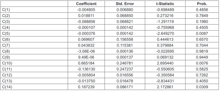
Table 5 shows the measure of the short run. C (1), also known as the error correction term, is negative and but insignificant as the p-value is 0.4875, which is more than 0.5, thus showing that an absence of long-term causatives

from independent variables to exchange rate. However, the negative coefficient suggests convergence but weak convergence towards equilibrium. The coefficients of C5 i.e., two-period lagged value of oil price and C 10, the one period lagged value of interest difference is substantial at a 1% level of significance. It denotes an association between exchange rate, oil prices, and interest difference.

Table 3: Cointegration

Hypothesized Trace 0.05 Max-Eigen 0.05

No. of C.E. (s) Statistic Critical Value Prob.** Statistic Critical Value Prob.**

None * 145.5366 95.75366 0.0000 68.48796 40.07757 0.0000

At most 1 77.04860 69.81889 0.0118 31.48954 33.87687 0.0939

At most 2 45.55907 47.85613 0.0809 22.37016 27.58434 0.2020

At most 3 23.18890 29.79707 0.2369 12.08459 21.13162 0.5393

At most 4 11.10431 15.49471 0.2052 10.10529 14.26460 0.2051

At most 5 0.999021 3.841466 0.3175 0.999021 3.841466 0.3175

*means rejection of the hypothesis at the 0.05 level

Table 4: Findings from VECM Exchange

Rate GDP Inflation Oil Price Interest

difference Money Supply Constant

1 −0.000116 27.98390 −0.006229 −1.090958 −0.001538 −45.73818

(0.00082) (3.22961) (0.05772) (0.68324) (0.00118)

[−0.14218] [ 8.66479] [−0.10792] [−1.59675] [−1.30373]

Table 5: System equation Coefficients

Coefficient Std. Error t-Statistic Prob.

C(1) -0.004805 0.006880 -0.698489 0.4856

C(2) 0.018811 0.068850 0.273216 0.7849

C(3) -0.088856 0.068821 -1.291119 0.1980

C(4) -0.000107 0.000142 -0.755968 0.4505

C(5) -0.000376 0.000142 -2.649270 0.0087

C(6) 0.069607 0.156558 0.444613 0.6570

C(7) 0.043832 0.115381 0.379884 0.7044

C(8) -3.08E-06 0.000136 -0.022695 0.9819

C(9) 9.49E-06 0.000137 0.069132 0.9449

C(10) 0.665184 0.246781 2.695440 0.0076

C(11) -0.136130 0.247237 -0.550605 0.5825

C(12) -0.005804 0.016556 -0.350584 0.7262

C(13) -0.013750 0.016478 -0.834431 0.4050

C(14) 0.187239 0.086171 2.172861 0.0309

Further Wald test has been performed to verify for short- run causality with the joint hypothesis of coefficients from C (4) to C (13) as 0. The Wald test has been conducted for testing the short-run causatives. The null hypothesis is; C(4)=

C(5)=C(6)=C(7)=C(8)=C(9)=C(10)=C(11)=C(12)=C(13)=0 which means that if the joint influence is zero, then there is no short-run causation to the exchange rate due to inflation, interest difference, GDP, money supply, oil price exists.

The chi-square statistic in Table 6 is 14.601. The related probability is 14 percent, which is more than 5 percent.

So the hypothesis of the absence of short-run causality is accepted at 5%. However, the probability value is 14.73 (not very far from 10%). So the individual analysis was also conducted to test that as to which variable may have a short- run causality.

The short-run causation test using Wald statistics shows a short-term association between oil price and interest difference and the dependent variable exchange rate. The other independent variables do not have either long or short-run causality towards the exchange rate. It means that there is short-term causation to the dependent variable from independent variables. Therefore it can be concluded that long and short-run causality is present in the model mentioned above. The results are similar to the study of Hosseini et al. (2011).

5. Conclusion

This study primarily focuses on verifying the fact that if the oil prices have any effect on the real exchange rate of the Indian economy. The model taken for the study is based on the economic rationale developed in the past, which suggests the inclusion of other macroeconomic variables such as GDP, inflation, the difference between the short term interest rate differences of the two countries under study, and inflation

along with actual oil prices. The results obtained through empirical analysis of the variables, as mentioned above, suggest that there is a dynamic association between oil prices and exchange rate as both the long run and short run causalities are confirmed. The insignificant error correction term has been found due to an insignificant association of exchange rate with money supply and GDP. The inclusion of these two is important as the exchange rate rationally should be related to the money supply in any economy, and the gross domestic product within the country.

The cointegration test suggested one cointegrating equation, which confirms a long-term association between exchange rate and inflation, interest difference, GDP, money supply, and oil price. The analysis reveals that crude oil value is negatively related to the exchange rate. The VECM model results show that the exchange rate measure through error correction is insignificant and negative. The study found weak convergence that could be due to other insignificant macroeconomic variables. The Wald statistic also indicates the short-run causation from the short-term interest rate and the prices of crude oil towards the exchange rate. The present study proves the incidence of a short-term and long-term causal association with the exchange rate from the short term interest rates and oil prices.

References

Alam, N. (2020). Do Oil Price Shock, and other Macroeconomic Variables Affect the Stock Market: A Study of The Saudi Stock Market. Humanities & Social Sciences Reviews, 8(3), 1234-1242. https://doi.org/10.18510/hssr.2020.83126

Amano, R. A., & Norden, S. (1998). Oil Prices and the Rise and Fall of the U.S. Real Exchange Rate. Journal of International Money and Finance, 17(2) 299-316. https://doi.org/10.1016/

S0261-5606(98)00004-7 Table 6: Wald Test

Test Name Test Value DF Probability

F-Test 1.460158 10,216 0.1560

Chi-square 14.60158 10 0.1473

Table 7: Wald Test

GDP MS Oil Price Inflation Interest diff

F-statistic 0.612449

(0.5430) 0.105106

(0.9003) 3.609222**

(0.0287) 0.002440

(0.997) 3.65972**

(0.0273)

Chi-square 1.224898

(0.5430) 0.210212

(0.9002) 7.218445**

(0.0271) 0.004880

(0.997) 7.3195**

(0.0257)

*The value in bracket represents the p-value at 5%

Basher, S. A., Haug, A. A., & Sadorsky, P. (2016). The impact of oil shocks on exchange rates: A Markov-switching approach. Energy Economics, 54, 11-23. doi.org/10.1016/j.

eneco.2015.12.004

Benhabib, A., Kamel, S, M., & Maliki, S. (2014). The Relationship between Oil Price and the Algerian Exchange Rate. Topics in Middle Eastern and African Economies, 16(1), 127-141.

Brahmasrene, T., Huang, J. C., & Sissoko, Y. (2014), Crude oil prices and exchange rates: Causality, variance decomposition and impulse response. Energy Economics, 44, 407-412.

DOI: 10.1016/j.eneco.2014.05.011

Coleman, S., Cuestas, J. C., & Mourelle, E. (2011). Investigating the oil price-exchange rate nexus: Evidence from Africa. Working Papers: 2011015. The University of Sheffield, Department of Economics.

Dogan, S., Ustaoglu, M., & Demez, S. (2012). Relationship between real oil price and real exchange rate: The case of Turkey.

Procedia - Social and Behavioral Sciences, 58(October), 1293- 1300. DOI: 10.1016/j.sbspro.2012.09.1112

Echchabi, A., & Azouzi, D. (2017). Oil Price Fluctuations and Stock Market Movements: An Application in Oman. The Journal of Asian Finance, Economics and Business, 4(2), 19-86. http://

dx.doi.org/10.13106/jafeb.2017.vol4.no2.1

Ghosh, S. (2011). Examining crude oil price: Exchange rate nexus for India during the period of extreme oil price volatility.

Applied Energy, 88(5), 1886-1889. doi.org/10.1016/j.

apenergy.2010.10.043

Hosseini, S. M., Ahmad, Z., & Lai, Y. (2011). The Role of Macro- economic Variables on Stock Market Index in China and India.

International Journal of Economics and Finance, 3(6), 233-243 Huang, Y., & Feng, G. (2007). The role of oil price shocks on

China’s real exchange rate. China Economic Review, 18(4), 403-416. https://doi.org/10.1016/j.chieco.2006.02.003

Johansen, S. (1988). Statistical Analysis of Cointegration Vectors.

Journal of Economic Dynamic and Control, 12(2), 231-254.

https://doi.org/10.1016/0165-1889 (88)90041-3

Jiranyakul, K. (2014). Does Oil Price Uncertainty transmit to the Thai Stock Market?, Journal of Economic and Financial Studies, 2(6), 16-25. http://doi.org/10.2139/ssrn.2450974 Lee, J. W., & Zhao, T. F. (2014). Dynamic Relationship between

Stock Prices and Exchange Rates: Evidence from Chinese Stock Markets. Journal of Asian Finance, Economics and Business, 1(1), 5-14. doi.org/10.13106/jafeb.2014.vol1.no1.5.

Krugman, P. (1980). Oil and the Dollar. Working Paper Series-554, National Bureau of Economic Research, Cambridge, MA.

https://www.nber.org/papers/w0554.pdf

Reboredo, J. C. (2012). Modelling Oil Price and Exchange Rate Co-movements. Journal of Policy Modeling, 34(3), 419-440.

https://doi.org/10.1016/j.jpolmod.2011.10.005

Reboredo, J. C., & Castro, M. (2013). A Wavelet Decomposition Approach to Crude Oil Price and Exchange Rate Dependence.

Economic Modelling, 32, 42-57. Doi.org/10.1016/j.econmod.

2012.12.028

Srivastava, A. (2017). A review on pricing of currency futures in Indian foreign exchange market. International Journal of Economics and Business Research, 13(2), 182-189. https://

dx.doi.org/10.1504/IJEBR.2017.082273

Tiwari, A. K., Mutascu, M. I., & Albulescu, C. T. (2013). The Influence of the International Oil Prices on the Real Effective Exchange Rate in Romania in a Wavelet Transform Framework.

Energy Economics, 40: 714-733. https://doi.org/10.1016/j.

eneco.2013.08.016

Nguyen, V. C., & Do, T. T. (2020). Impact of Exchange Rate Shocks, Inward FDI and Import on Export Performance: A Cointegration Analysis. Journal of Asian Finance, Economics and Business, 7(4), 163-171. https://doi.org/10.13106/jafeb.2020.vol7.

no4.163

Lv, X., Lien, D., Chen, Q., & Yu, C. (2018). Does exchange rate management affect the causality between exchange rates and oil prices? Evidence from oil-exporting countries.

Energy Economics, 76, 325-343. https://doi.org/10.1016/j.

eneco.2018.10.017