DOI : 10.5394/KINPR.2010.34.9.719
Operational Performance Evaluation of Korean Major Container Terminals
Bo LU†․Nam-Kyu Park*
†Department of Distribution Management, TongMyong University, Busan 608-711, Korea
*Faculty of Port Logistics, TongMyong University, Busan 608-711, Korea
Abstract : As the competition among the container terminals in Korea has become increasingly fierce, every terminal is striving to increase its investments constantly and lower its operational costs in order to maintain the competitive edge and provide satisfactory services to terminal users. The unreasoning behavior, however, has induced that substantial waste and inefficiency exists in container terminal production. Therefore, it is of great importance for the terminal to know whether it has fully used its existing infrastructures and that output has been maximized given the input. From this perspective, data envelopment analysis (DEA) provides a more appropriate benchmark. This study applies three models of DEA to acquire a variety of analytical results about the operational efficiency to the Korean container terminals. According to efficiency value analysis, this study first finds the reason of inefficiency. It is followed by identification of the potential areas of improvement for inefficient terminals by applying slack variable method and giving the projection results. Finally, return to scale approach is used to assess whether each terminal is in a state of increasing, decreasing, or constant return to scale. The results of this study can provide terminal managers with insight into resource allocation and optimization of the operating performance.
Key words : Efficiency, Korean major container terminals, Data envelopment analysis, Throughput, Performance
†Corresponding author, [email protected] 051) 629-1861
* [email protected] 051)629-1861
1. Introduction
In recent years, with rapid expansion of global business and international trade, one distinctive feature of the current container terminal industry is that competition among container terminals is more intensive than previously (Liu, 1995; Tongzon and Heng, 2005; Yap and Lam, 2005).
To maintain its competitiveness in such competitive condition, Kevin Cullinane et al. (2006) claimed container terminals have to invest heavily in sophisticated equipment or in dredging channels to accommodate the most advanced and largest container ships in order to facilitate cost reductions for the container shipping industry.
It is important to note, however, that pure physical expansion is constrained by a limited supply of available land, especially for urban centre terminals, and escalating environmental concerns. In addition, the excessive and inappropriate investment also can induce the phenomenon of inefficiency and wasting of resources. In this context, improving the productive efficiency of container terminals (Le-Griffin et al., 2006) appears to be the viable solution.
Realizing the facts, Korean port authorities like BPA, IPA, and UPA have shown strong interest in efficient terminal management. Thus, they are continually searching for strategies to meet growing demands by utilizing their
resources reasonably.
For a container terminal, productivity performance makes significant contribution to the prospects of survival and competitive advantage. Traditionally, the productivity of container terminals has been variously evaluated by numerous attempts at calculating and seeking to improve or optimize the operational productivity of cargo-handling at berth and in the container yard (Kim, 1997; Kim and Bae, 1998; Kim and Kim, 1998; Kim and Kim, 1999; Robinson, 1999; Avriel et al., 2000; Wilson and Roach, 2000; Chu and Huang, 2002).
If Korean container terminals can conduct effective evaluation of their operational performance in a globally competitive environment, it will provide valuable information for terminal management in their attempts to establish competitive strategies and to improve their resource efficient utilization.
From this perspective, data envelopment analysis model
provides a more appropriate benchmark for the container
terminal. The aim of this study is to evaluate the operational
performance of container terminals which can be calculated
by relative productivity, and defined as how to minimize
inputs while producing a given level of output, or how to
maximize outputs while using no greater quantity of any of
the individual inputs within a given set of inputs, by
applying with DEA-CCR, DEA-BCC, and DEA-Super Efficiency, three models to acquire a variety of analytical results about the productivity efficiency for thirteen Korean major container terminals.
According to efficiency value analysis, this study first finds the reason of inefficiency. It is followed by identification of the potential areas of improvement for inefficient terminals by applying slack variable method which includes the projection analysis. Finally, return to scale approach is used to assess whether each terminal is in a state of increasing, decreasing, or constant return to scale.
The paper is structured as follows: after the introductory section of chapter 1, there will be followed by the description of three data envelopment analysis (DEA) models. In so doing, the three main approaches to applying DEA to analyze data are included in chapter 2. The required input and output variables are defined and the data that has been collected is described. Efficiency estimates of the study object are derived in chapter 3. Finally, conclusions are drawn in chapter 4.
2. Research method
2.1 Data envelopment analysis (DEA)
DEA can be roughly defined as a non-parametric method of measuring the efficiency of a Decision Making Unit (DMU) with multiple inputs and/or multiple outputs. This is achieved by constructing a single ‘virtual’ output to a single
‘virtual’ input without pre-defining a production function.
The term DEA and the CCR model were first coined in Charnes et al. (1978) and were followed by a phenomenal expansion of DEA in terms of its theory, methodology and application over the last few decades. The influence of the CCR paper is reflected in the fact that by 1999 it had been cited over 700 times (Forsund and Sarafoglou, 2002).
Among the models in the context of DEA, the two DEA models, named CCR (due to Charnes et al., 1978) and BCC models (due to Banker et al., 1984) have been widely applied. The CCR model assumes constant returns to scale so that all observed production combinations can be scaled up or down proportionally. The BCC model, on the other hand, allows for variable returns to scale and is graphically represented by a piecewise linear convex frontier.
Because the CCR model gives a value of 1 for all efficient DMUs, it is unable to establish any further distinctions among the efficient DMUs. Andersen and Petersen, therefore, presented a new DEA model, DEA-Super
Efficiency model. This model removes an efficient DMU, and then estimates the production frontier again; this provides a new efficiency value for the efficient DMU that had previously been removed. The new efficiency value can thus be greater than 1. However, if an inefficient DMU is removed, the original production frontier does not change.
Therefore, the efficiency values of inefficient DMUs do not change in the DEA-Super Efficiency model.
In other words, the two basic models of DEA (i.e. CCR and BCC models) are used to provide the efficiency values for self-appraisal of terminal operational performance. The DEA-Super Efficiency model is used to make further distinctions among the efficient DMUs since they all have efficiency values of 1 in the CCR model. Thus, the varied and complementary information can be extracted from these three models to provide a more complete and comprehensive performance evaluation.
The DEA methodology has been applied to the evaluation of terminal performance in the previous literature. For example, Roll and Hayuth (1993) probably represents the first work to advocate the application of the DEA technique to the terminals context. However, it remains a purely theoretical exposition, rather than a genuine application. For the period 1990–1999, Itoh (2002) conducted a DEA window analysis using panel data relating to the eight international container ports in Japan. Tongzon (2001) uses both DEA-CCR and DEA-Additive models to analyze the efficiency of four Australian and 12 other international container ports for 1996. Barros and Athanassiou (2004) apply DEA to the estimation of the relative efficiency of a sample of Portuguese and Greek seaports.
However, most previous studies have adopted two basic models of DEA (the CCR model and the BCC model) to obtain aggregate efficiency, pure technical efficiency and scale efficiency. In contrast, this study also adopts DEA-Super Efficiency to acquire useful and complementary information about terminals.
In this study, the DEA model includes three types of
analysis. With respect to the efficiency value analysis, when
technical efficiency is less than 1, that is technical
inefficient, this means that the efficiency of the inputs and
output being used is not appropriate, and that it is necessary
to decrease input or/and increase output. However, when the
scale efficiency is less than 1, that is scale inefficient, it
means that the operational scale is not achieving an optimal
value, and that the operational scale should be enlarged or
reduced (based on the return to scale). In addition, it is
possible to compare the technical efficiency value with the scale efficiency value, with the smaller value of the two indicating the major cause of inefficiency. Finally, the slack variable analysis handles the utilization rate of input and output variables. It does this by assessing how to improve the operational performance of inefficient DMUs by indicating how many inputs to decrease, and/or how many outputs to increase, so as to render the inefficient DMUs efficient. This facilitates an overall understanding of which input variable is more critical for efficiency improvement (L.
C. LIN, 2007). In summary, the flow process of multiple DEA analyses can be depicted as shown in figure 1.
Return to scale Slack variable
approach Efficiency value analysis
Efficient < 1
Scale efficiency and pure technical efficient
No improvement
Constant Cause inefficiency
Increasing Scale efficiency >
technical efficiency
Scale efficiency <
technical efficiency
Scale inefficient
Pure technical inefficient
Need improvement Inefficient < 1
Decreasing
DEA efficiency values of DMUs
Fig. 1 Flow process of DEA analysis
Source: Modified by L. C. Lin and C. C. Tseng, 2007
2.2 Research procedure
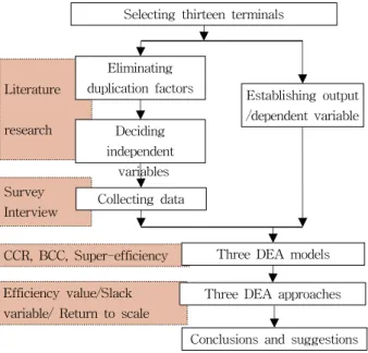
The research procedure of this study is summarized in figure 2. After the selection of container terminals, the output variable for the study should be selected firstly.
Drawing on the literature review, site survey & interview, and Brainstorming to eliminate the duplication factors, the initial inputs variables can be chosen.
Then, in order to provide a more comprehensive picture of research, and for the purpose of finding the operational efficiency value, an exploration composed of the CCR, BCC and Super-efficiency DEA models and three analytical approaches which include efficiency value analysis, slack variable method and return to scale approach have been applied. After that, the evaluation results and suggestions will be given.
Efficiency value/Slack variable/ Return to scale Survey
Interview Literature
research
Selecting thirteen terminals
Eliminating duplication factors
Deciding independent
variables Collecting data
Establishing output /dependent variable
CCR, BCC, Super-efficiency Three DEA models
Three DEA approaches
Conclusions and suggestions
Fig. 2 Research procedure
Source: Authors of the original source
3. Result analysis
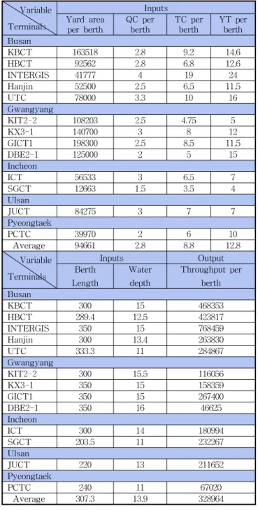
3.1 Data collection and definitions of variables Because it is difficult to acquire data on integral scale, most of the previous documents have focused on the evaluation of several major terminals over the years. For doing a typical and deep analysis, the object of study comprises the thirteen Korean major container terminals, almost contain all of the Korean major container terminals, including KBCT, HBCT, INTERGIS, Hanjin, UTC terminal in Busan port, KIT2-2, KX3-1, GICT1, DBE2-1 terminal in Gwangyang port, ICT, SGCT terminal in Incheon port, JUCT terminal in Ulsan port and PCTC terminal in Pyeongtaek port. When June 20th, 2009, the questionnaire has been made such as table 1 and sent to the relative departments of 13 container terminals, after receiving the questionnaire answers. The researchers of this study went to the 13 terminals to confirm the accuracy of the data during July 25th, 2009 to August 30th, 2009.
With respect to definitions of variables, a thorough
discussion of the importance, difficulties and potential impact
of variable definition can be found in (Song et al, 2003), and
the main criterion of this study for choosing variables can be
summarized as that the input and output variables should
reflect the actual objectives and process of container terminal
production as accurately as possible. Because the most
container terminals rely heavily upon sophisticated equipment
and information technology, rather than being intensive labour.
Berth
Throughput (TEU) Water
Depth(m) Berth
Length(m) Berth No.
Crane No.
Type No.
Yard Yard
Area (㎡)
CFS Area (㎡)
Crane No. Gate No.
RTGC RMGC RS YT In Out
Table 1 Questionnaire of study
Therefore, in order to determine the input variables, the adopted initial variables in the study are discovered through an abundant literature review, discussion with experts working in container ports for more than 20 years and brainstorming, almost factors that relevant to terminal operation are to be considered such as terminal facilities like yard area, number of berth, water depth, length of berth, gate, rail station etc., and port equipment like Y/T, Q/C, RTGC, RMGC, reach stacker, top handler and folk lifter etc.
However, in the light of concerning the process of container terminal production lie on crucially the efficient utilization of infrastructures and facilities. The yard area, the quantities of quay crane, yard crane, yard tractor, berth length, and water depth have been deemed to be the most suitable input variables.
Fig. 3 Definitions of input variables Source: Authors of the original source
With regard to the output variable, container throughput is unquestionably the most important and widely accepted indicator of container terminal output. Almost all previous studies treat it as an output variable, because it closely relates to the need for cargo-related facilities and services and is the primary basis upon which container terminals are compared, especially in assessing their relative size, investment magnitude or activity levels. Most importantly, it also forms the basis for the revenue generation of a container port or terminal (Kevin Cullinane et al, 2005).
Synthesizing the former research, in this study, the output variable is defined as throughput.
Variable Terminals
Inputs Yard area
per berth
QC per berth
TC per berth
YT per berth Busan
KBCT 163518 2.8 9.2 14.6
HBCT 92562 2.8 6.8 12.6
INTERGIS 41777 4 19 24
Hanjin 52500 2.5 6.5 11.5
UTC 78000 3.3 10 16
Gwangyang
KIT2-2 108203 2.5 4.75 5
KX3-1 140700 3 8 12
GICT1 198300 2.5 8.5 11.5
DBE2-1 125000 2 5 15
Incheon
ICT 56533 3 6.5 7
SGCT 12663 1.5 3.5 4
Ulsan
JUCT 84275 3 7 7
Pyeongtaek
PCTC 39970 2 6 10
Average 94661 2.8 8.8 12.8
Variable Terminals
Inputs Output
Berth Length
Water depth
Throughput per berth Busan
KBCT 300 15 468353
HBCT 289.4 12.5 423817
INTERGIS 350 15 768459
Hanjin 300 13.4 263830
UTC 333.3 11 284867
Gwangyang
KIT2-2 300 15.5 116056
KX3-1 350 15 158359
GICT1 350 15 267400
DBE2-1 350 16 46625
Incheon
ICT 300 14 180994
SGCT 203.5 11 232267
Ulsan
JUCT 220 13 211652
Pyeongtaek
PCTC 240 11 67020
Average 307.3 13.9 328964
Table 2 Data collection of Korean major terminals
Source: First-hand data collected by authors
3.2 Standardization of Output and Input Variables In order to gain the accurate performance of container terminals, the value of input and output variables should be standardized.
Therefore, this study defines the inputs and output of
each container terminal at the level of per berth which is
applied with the published data by inner report, except the
input of water depth still keeping the actual values. The
standardization formula can be summarized as:
3.3 Efficiency results derived from DEA models As with using the data of thirteen Korean container terminals by applying with DEA approaches, for proving the production function of container terminals exhibits either constant or variable returns to scale, the DEA-CCR and DEA-BCC models are chosen from among several DEA models to analyze terminal production. In addition, for ordering the efficiency terminals, the DEA-Super efficiency is adopted.
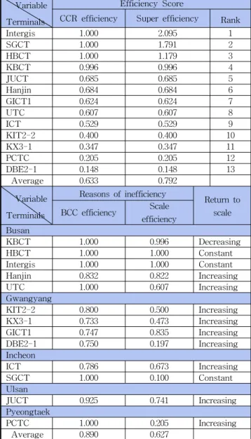
The efficiency analytical results for container terminals are summarized in table 3, and the following observations can be made. The column and row totals represent, respectively, the efficiency value of each terminal and the condition of return to scale in 2008 year.
It is clear from table 3 that, the DEA-CCR model yields lower average efficiency estimates than the DEA-BCC model, with respective average values of 0.633 and 0.792, where an index value of 1.000 equates to perfect (or maximum) efficiency. The Super-efficiency model was utilized to reinforce the discriminatory power of the CCR model. INTERGIS has the best performance among these thirteen terminals. SGCT and HBCT terminal ranked as the second and third best in this model respectively. The scores are more than 1.100, with these efficiency values far exceeding that of other terminals.
By using of efficiency value analysis, slack variable approach, and return to scale method, the analytical results can be summarized as:
Firstly, the aggregate efficiency value acquired from the CCR model of HBCT, INTERGIS, and SGCT are all equal to 1. The efficiency values of other container terminals in 2008 are less than 1, which indicate that they were relatively inefficient container terminals. The pure technical efficiency value obtained from the BCC model represents the efficiency in terms of the usage of input resources. If a terminal has an efficiency value equal to 1 in the CCR model, the value of its pure technical efficiency would also be equal to 1.
However, if the efficiency value on the CCR model is less than 1, a comparison could be made between the pure technical efficiency value and the scale efficiency value, thus allowing a judgement to be made about whether the inefficiency is caused by an inefficient application of input
resources or an inappropriate production scale.
Variable Terminals
Efficiency Score
CCR efficiency Super efficiency Rank
Intergis 1.000 2.095 1
SGCT 1.000 1.791 2
HBCT 1.000 1.179 3
KBCT 0.996 0.996 4
JUCT 0.685 0.685 5
Hanjin 0.684 0.684 6
GICT1 0.624 0.624 7
UTC 0.607 0.607 8
ICT 0.529 0.529 9
KIT2-2 0.400 0.400 10
KX3-1 0.347 0.347 11
PCTC 0.205 0.205 12
DBE2-1 0.148 0.148 13
Average 0.633 0.792
Variable Terminals
Reasons of inefficiency
Return to scale BCC efficiency Scale
efficiency Busan
KBCT 1.000 0.996 Decreasing
HBCT 1.000 1.000 Constant
Intergis 1.000 1.000 Constant
Hanjin 0.832 0.822 Increasing
UTC 1.000 0.607 Increasing
Gwangyang
KIT2-2 0.800 0.500 Increasing
KX3-1 0.733 0.473 Increasing
GICT1 0.747 0.835 Increasing
DBE2-1 0.750 0.197 Increasing
Incheon
ICT 0.786 0.673 Increasing
SGCT 1.000 0.100 Constant
Ulsan
JUCT 0.925 0.741 Increasing
Pyeongtaek
PCTC 1.000 0.205 Increasing
Average 0.890 0.627
Table 3 Efficiency under three DEA models
All of the pure technical efficiency values of KBCT, HBCT, INTERGIS, UTC, SGCT, and PCTC are equal to 1.
The technical efficiency values of other container terminals are less than 1, thus indicating that they would need to improve their usage of resources. Among these, KX3-1 has the least pure technical efficiency value.
Secondly, according to the results of return to scale,
HBCT, INTERGIS and SGCT were relatively efficient
container terminals and had constant return to scale. In
addition, apart from constant return to scale, Hanjin, UTC,
KIT2-2, KX3-1, GICT1, DBE2-1, ICT, JUCT and PCTC
were in a state of increasing return to scale; only KBCT
was decreasing return to scale in 2008.
Variable Terminals
Inputs
Yard area/berth QC per berth TC per berth Busan
KBCT 115623.6 0 0
HBCT Intergis
Hanjin 0 0.03 0
UTC 13488.61 0.36 0
Gwangyang
KIT2-2 36925.04 0.25 0.15
KX3-1 27281 0.05 0
GICT1 109264.6 0 0
DBE2-1 15970.5 0 0
Incheon
ICT 20047.35 0.47 0.31
SGCT Ulsan
JUCT 46242.17 0.79 0.81
Pyeongtaek
PCTC 1389.23 0 0
Average 29710.16 0.15 0.09
Variable Terminals
Inputs
YT per berth Berth length Water depth Busan
KBCT 1.95 0 0.81
HBCT Intergis
Hanjin 1.18 14.27 0
UTC 0.98 47.12 0
Gwangyang
KIT2-2 0 18.24 0.7
KX3-1 0 11.32 0
GICT1 0.72 39.95 0.39
DBE2-1 1.36 12.63 0.27
Incheon
ICT 0 17.74 0
SGCT Ulsan
JUCT 0 0 1.18
Pyeongtaek
PCTC 0.36 2.88 0
Average 0.50 12.63 0.26
Table 4 Slack variable analysis results
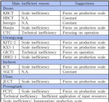
Finally, the slack variable analysis showed, in table 4, that HBCT, INTERGIS, Hanjin, SGCT and PCTC had been relatively efficient; their ratios of input variables to output variable were appropriate, and they were capable of applying their input resources effectively to achieve enhanced efficiency. In contrast, KBCT, UTC, KIT2-2, KX3-1, GICT1, DBE2-1, ICT and JUCT were relatively inefficient as a result of inappropriate application of input resources.
Furthermore, in these cases, an inappropriate production scale is the cause of the inefficiency of KBCT, KIT2-2, KX3-1, DBE2-1, ICT and JUCT; while UTC and GICT1 were caused by technical inefficiency. The results indicated that main inefficient reason of Korean container terminals
should adjust the yard area and increase the throughput.
The specific analysis results have been summarized as table 5.
Main inefficient reason Suggestions Busan
KBCT Scale inefficiency Focus on production scale
HBCT N.A. Constant
Intergis N.A. Constant
Hanjin Scale inefficiency Focus on production scale UTC Technical inefficiency Focusing on operation Gwangyang
KIT2-2 Scale inefficiency Focus on production scale KX3-1 Scale inefficiency Focus on production scale GICT1 Technical inefficiency Focus on operation DBE2-1 Scale inefficiency Focus on production scale Incheon
ICT Scale inefficiency Focus on production scale
SGCT N.A. Constant
Ulsan
JUCT Scale inefficiency Focus on production scale Pyeongtaek
PCTC Scale inefficiency Focus on production scale Technical inefficiency : Inefficient application of input resources Scale inefficiency: Inappropriate production scale
Table 5 Implication of analysis
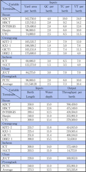
After finding out the inefficient reasons, the inefficient terminal should make an adjustment to reach efficient performance. By applying with the projection analysis, this study can identify the optimal benchmark of the quantities of input and output variables. The results has been summarized on table 6.
4. Conclusions
For container terminals in the competitive circumstances,
efficiency is an important concept and concerned with how
to use limited resources more economically for any sort of
production. As a benchmarking approach to study efficiency,
DEA enables a container terminal to evaluate its
performance from each other in DMUs. By doing this, the
possible waste of resources and the industry best practice
can be identified. By using a range of DEA models, this
study has evaluated the thirteen Korean container terminals,
and in the process has acquired varied and complementary
conclusions from the different models. The study has
making efficiency value analysis, and has established a
return to scale to compare the technical efficiency value
with the scale efficiency value, with the lesser of the two
indicating the major cause of inefficiency for each container
terminal. Moreover, using slack variable analysis, the study
has provided useful information that indicates how relatively inefficient container terminals can improve their efficiency.
Variable Terminals
Inputs Yard area
per berth
QC per berth
TC per berth
YT per berth Busan
KBCT 162,750.0 4.0 19.0 24.0
HBCT 125,745.5 2.8 9.2 14.2
INTERGIS 129,400.0 2.8 6.8 12.6
Hanjin 96,000.0 2.0 6.0 10.0
UTC 74,000.0 2.5 6.5 11.5
Gwangyang
KIT2-2 105,535.7 2.3 7.9 12.0
KX3-1 106,509.2 1.8 5.0 7.6
GICT1 103,151.8 2.2 7.4 11.5
DBE2-1 175,600.0 2.0 3.8 4.0
Incheon
ICT 68,886.0 3.0 6.5 7.0
SGCT 122,273.0 1.5 3.5 4.0
Ulsan
JUCT 84,275.0 3.0 7.0 7.0
Pyeongtaek
PCTC 96,000.0 2.0 6.0 10.0
Average 111,548.20 2.5 7.3 10.4
Variable Terminals
Inputs Output
Berth Length
Water depth
Throughput per berth Busan
KBCT 350.0 15.0 768,459.0
HBCT 286.5 12.6 475,349.0
INTERGIS 289.4 12.5 420,594.0
Hanjin 240.0 11.0 355,991.0
UTC 300.0 13.4 279,569.0
Gwangyang
KIT2-2 255.7 11.6 414,915.0
KX3-1 225.4 11.0 219,503.4
GICT1 251.8 11.4 400,184.0
DBE2-1 390.0 15.5 51,638.0
Incheon
ICT 300.0 14.0 172,448.0
SGCT 203.5 11.0 14,772.0
Ulsan
JUCT 220.0 13.0 169,952.0
Pyeongtaek
PCTC 240.0 11.0 355,991.0
Average 273.3 12.5 315,335.8