https://doi.org/10.1007/s40042-021-00123-0 ORIGINAL PAPER
Statistical property of record breaking events in the Korean housing market
Jinho Kim1 · Soon‑Hyung Yook2
Received: 22 January 2021 / Revised: 17 February 2021 / Accepted: 19 February 2021
© The Korean Physical Society 2021
Abstract
We study the record statistics in the Korean housing market. To characterize the statistical properties of records, we analyze the record rate and the expected number of records for the transaction price of apartments and the volatility. From the numeri- cal analysis, we find that the record rate of price in the overheated region is well described by the record rate obtained from the symmetric independent and identically distributed (IID) random sequence when the price change is relatively small. On the other hand, during the period for the subprime mortgage crisis, the record rate of price in the overheated regions is well approximated by that for the correlated sequence. More interestingly, when the price continuously increases the record rate of price shows a strong seasonal effect in the overheated region, while that in the normal region is simply described by the symmetric IID random sequence with constant drift on the average.
Keywords Record statistics · Extreme value statistics · Extreme events in housing markets · Econophysics
1 Introduction
Record statistics are the statistics on the record values or the record-breaking events. A record is an entry in discrete time series that is larger (an upper record) or smaller (a lower record) than all preceding entries [1–6]. Thus, the record sta- tistics are closely related to the extreme value statistics [7].
In record statistics, two interesting questions might be (1) how many records occur for a given time interval? and (2) how long does it survive? To answer such questions, various statistical properties of records, for example, the distribu- tion of the number of records and the distribution of the age of the longest record, are investigated [5]. Such statistical properties of records have been widely studied in various scientific disciplines such as meteorology [8–10], biology [11], sports [12, 13], and economics [14], due to its public interests such as climate change and theoretical importance to understand the underlying evolutionary dynamics [15, 16].
Analytical and numerical studies have uncovered many interesting characteristics of record statistics. For example, the mean number of the records in a sequence of random variables with distributions that broaden or sharpen with time was investigated, and it was found that the mean num- ber of records shows different asymptotic behaviors for three distributions (Fréchet, Gumbel, and Weibull distributions) [1]. It was also shown that the record statistics of a time series generated by a continuous and symmetric Markov process is not affected by the details of the distribution [3].
The effect of measurement error and noise on record sta- tistics was also studied [17]. More recently, the long-range correlation between record events in the Bernoulli process was also investigated to describe the precipitation data [18].
The effect of drift velocity on the record rate and the order- ing probability was also analytically studied with a close relationship to the global temperature change [2]. The result was successfully showed that the current rise in the mean temperature affects the rate of occurrence of the temperature record [19]. Thus, the record statistics have also provided a useful theoretical framework to analyze the observed phe- nomena in nature ranging from climate changes such as the increasing trend of temperature [9] and amount of rainfall from the precipitation time series [18] to the earthquake analysis [20].
Print ISSN 0374-4884
* Soon-Hyung Yook [email protected]
1 Department of Social Network Science, Kyung Hee University, Seoul 02447, South Korea
2 Department of Physics and Research Institute for Basic Sciences, Kyung Hee University, Seoul 02447, South Korea
Due to a large amount of available data, various financial systems are studied in statistical physics as a part of complex systems in which human activity causes rich interesting phe- nomena [21, 22]. Many studies have shown that the financial systems share some common universal features such as the fat-tailed distribution of income for individuals or firms, return in the stock exchange market [23, 24] and foreign exchange market [25, 26], and high-order correlations in price changes [27, 28]. However, the record statistics in the financial systems are rarely understood. In financial markets, sellers want to sell their items at the highest price, while the buyers eager to buy at the lowest price. Since the highest (lowest) price is the upper (lower) record in the time series of the price change, uncovering the underlying statistical property of records in financial data has also great impor- tance to understand the market dynamics [29–31].
The housing market is one of the very important finan- cial markets. Recently, the universal behaviors of the house prices for major cities in developed countries were inves- tigated based on the macroscopic data [32–34]. However, the statistical and dynamical properties based on the micro- scopic data are rarely studied. The housing market also inter- acts with various exogenous economic factors such as GDP, interest rates, inflation rates, tax policies, etc. [35–38], and shares the common universal properties with other financial markets [39]. In the housing market, the sellers and buyers behave in the same fashion as those in other financial sys- tems. Furthermore, the price of real estate slowly changes compared with the price of other financial items such as stocks and currency. Therefore, finding the exogenous effect on the market dynamics and analyzing the relationship between elements in the market might be easier than other financial systems. In this sense, understanding the record statistics in the housing market is also very important to investigate its effect on the global financial system.
In this paper, we numerically analyze record statistics of price and volatility in the Korean housing market. We use the Korean housing market data from 1 Jan. 2006 to 31 Dec.
2018, and select 110 cities and Gus (mid-size administrative districts in Korea). From the data, we find that the measured average record rate for prices strongly affected by exogenous effects, such as economic crisis comes from the outside the market and seasonal effect. On the other hand, the record statistics of logarithmic return are well described by the sim- ple symmetric independent and identically distributed (IID) random sequence.
2 Dataset
To study the record statistics in the Korean housing market, we use the “real estate price list” data from the open data portal of the National Information Society Agency from 1
Jan. 2006 to 31 Dec. 2018 [40]. The apartment is the most popular residential type in Korea. Thus, we focus only on the apartment trading data. Since most of the population resides in the urban area in Korea, we select only the transaction data for the urban area. Here we use two types of Korean administrative districts for the urban area. “Si”-district is a general type of urban area which corresponds to a city.
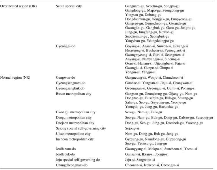
Besides, metropolitan cities in Korea such as Seoul can be divided into smaller mid-size administrative districts, “Gu”- districts. The population of the Gu-district is comparable to the Si-district. Therefore, we define the urban area as the Si-district and the Gu-district for metropolitan cities. Based on the act for Korean housing [41] and Urban Planning Sta- tus 2019 data from Korean Statistical Information Service [42], we choose 110 administrative districts (Sis and Gus) which satisfy the following conditions: (i) the population of Si or Gu should be larger than 100,000, and (ii) the fraction of the population in the citified area is more than 80% of the total population. The 110 districts are grouped into two dif- ferent regions depending on the trading patterns in housing markets [43]. The urban area in Seoul and Gyeonggi-do (the nearest province from Seoul) is grouped as the overheated region (OR), while the rest of the urban area is classified as the normal region (NR). Each group and corresponding administrative districts are listed in Table 1.
For numerical analysis, we use the average price per square meter of a given district from transaction data. The data contains the transaction record for every 10 days. Thus, the unit time step in the following analysis corresponds to 10 days. Let Yi(n) be the average price of apartment in an administrative district i at time step n. If there is no transac- tion in a district i at time step n, we assume that the average price is unchanged, i.e. Yi(n) = Yi(n − 1) . From the obtained time series {Yi(n)} for each district i, the logarithmic return of Yi(n) is defined as
where Δn = 1 . The volatility is defined as 𝜎i≡��
��
𝜌i(n)−⟨𝜌i(n)⟩
𝜎𝜌
��
�� , where 𝜎𝜌 indicates the standard deviation of the return for a given period [44, 45].
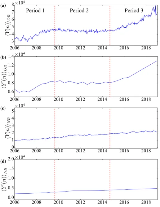
In Fig. 1a we show the measured ⟨Y(n)⟩OR in Seoul as an example of the average price change in OR. Here
⟨...⟩G denotes the average over the mid-size administra- tive districts in the group G (OR or NR). Based on the behavior of ⟨Y(n)⟩OR , we divide the time series into three distinctive periods (see the vertical dotted lines in Fig. 1). The boundary of each period is determined by the pattern of ⟨Y(n)⟩OR because more than half of Koreans reside in the OR including Seoul and its gross regional domestic product (GRDB) amounts to 50%
GDP of Korea [42]. In order to remove some additional effects, we use the detrending method suggested by Ref.
(1) 𝜌i(n) = ln(Yi(n)) − ln(Yi(n − Δn)),
[46]. In Fig. 1b we display the average detrended price for Seoul. The average detrended price is defined as
⟨Y�(n)⟩G=⟨Y(n)⟩G−�
sw(n) + sm(n) + sy(n) + 𝜖n� , where sw(n) , sm(n) and sy(n) are the standard Fourier series with different period P = 7 , 30 and 365.25, respectively. These values of P correspond to weakly, monthly, and yearly trends of price. 𝜖n denotes an error representing any idio- syncratic changes that are not accommodated by the model (see Ref. [46] for details). The behavior of ⟨Y�(n)⟩OR is nearly identical with that of ⟨Y(n)⟩OR . Therefore, ⟨Y�(n)⟩OR shares the same criteria with ⟨Y(n)⟩OR for the division of the given time interval as shown in Fig. 1b. A slight devia- tion of the boundary from those in Fig. 1a, b does not affect the results. Each period is labeled with period I, II, or III. Period I (1st. Jan. 2006–1st. Jan. 2009) con- tains global economic crisis originated from the subprime
mortgage crisis in the US [47]. As an indirect effect of subprime mortgage crisis, the price of an apartment in Korea increased during period I1. In period II (1st. Sep.
2009–11st. Sep. 2014), ⟨Y(n)⟩OR fluctuates around some fixed constant price, which corresponds to the quiescent period without any big economic event. In period III (11th.
Sep. 2014–21st. Dec. 2018), ⟨Y(n)⟩OR sharply increases due to the mitigating policy of the Korean government to activate the housing market. Therefore, we expect that the record statistics in each period should be distinctive. In
Table 1 The list of two different groups in Korea based on the trading pattern
The name of the metropolitan city or province (do-district) is listed in the second column. The name of Si or Gu district is listed in the third col- umn
Over heated region (OR) Seoul special city Gangnam-gu, Seocho-gu, Songpa-gu
Gangdong-gu, Mapo-gu, Seongdong-gu Yongsan-gu, Dobong-gu
Dongdaemun-gu, Dongjak-gu, Eunpyeong-gu Gangseo-gu, Geumcheon-gu, Gwanak-gu Gwangjin-gu, Gangbuk-gu, Guro-gu, Jongro-gu Jung-gu, Jungrang-gu, Nowon-gu
Seodaemun-gu , Seongbuk-gu Yangchun-gu, Yeongdeungpo-gu
Gyeonggi-do Goyang-si, Ansan-si, Suwon-si, Uiwang-si
Hwaseong-si, Bucheon-si, Pyeongtaek-si Gwangmyeong-si, Guri-si, Seongnam-si Anyang-si, Namyangju-si, Siheung-si Osan-si, Hanam-si, Uijeongbu-si, Paju-si Gwangju-si, Gunpo-si, Gimpo-si Yongin-si, Yangju-si
Normal region (NR) Gangwon-do Gangneung-si, Wonju-si, Chuncheon-si
Gyeongsangnam-do Gimhae-si, Yangsan-si, Jinju-si, Changwon-si Gyeongsangbuk-do Gyeongsan-si, Gyeongju-si, Gumi-si, Pohang-si Busan metropolitan city Gangseo-gu, Geumjeong-gu, Gijang-gu, Nam-gu
Dongnae-gu, Busanjin-gu, Buk-gu, Sasang-gu Saha-gu, Seo-gu, Suyeong-gu, Yeonje-gu Yeongdo-gu, Jung-gu, Haeundae-gu Gwangju metropolitan city Seo-gu, Nam-gu, Buk-gu
Daegu metropolitan city Seo-gu, Nam-gu, Buk-gu, Dong-gu, Dalseo-gu, Suseong-gu Daejeon metropolitan city Dong-gu, Seo-gu, Jung-gu, Daedeok-gu, Yuseong-gu Sejong special self-governing city Sejong-si
Ulsan metropolitan city Nam-gu, Dong-gu, Buk-gu, Jung-gu Incheon metropolitan city Gyeyang-gu, Namdong-gu, Bupyeong-gu
Seo-gu, Yeonsu-gu, Jung-gu
Jeollanam-do Gwangyang-si, Mokpo-si, Suncheon-si, Yeosu-si
Jeollabuk-do Gunsan-si, Iksan-si, Jeonju-si
Jeju special self-governing do Jeju-si, Seogwipo-si
Chungcheongnam-do Cheonan-si, Jecheon-si, Cheongju-si
1 We also check the raw transaction price data in each district for period I. From the data we find that the price of the apartment in every district in OR shows almost the identical behavior with Fig. 1a or b. Thus, the continuously increasing behavior for period I is not originated from the numerical artifact such as averaging or detrending of the data.
Fig. 1c, d, we display ⟨Y(n)⟩NR and ⟨Y�(n)⟩NR , respectively.
The data shows that ⟨Y(n)⟩NR and ⟨Y�(n)⟩NR for NR con- tinuously increases for the entire period of investigation.
3 Methods for record statistics analysis
In this section, we summarize the analytical results for record statistics which are used in our analysis. For a sequence of random variable {xn} drawn from a given dis- tribution f(x), the expected number of record at step n, Rn , has been analytically obtained when f(x) is characterized by some well-known distributions such as Gaussian [1–6]. For simplicity, we use the indication function first introduced in Ref. [18]. The indication function, In at step n is defined as
If we have D different sequences, {xi,n} (i = 1, … , D) , then we obtain D indication functions from the sequences. The record rate ⟨In⟩ that a record occurs at step n is defined as
In our housing market data, D corresponds to the total num- ber of districts in each regional group, and xi,n represents Yi,n , 𝜌i,n , or 𝜎i,n for district i at nth time step. From Eqs. (2) and (3), the expected number of record, Rn , is defined as [18]
(2) In=
{1 if record breaking event occurs in the n-th step, 0 otherwise.
(3)
⟨In⟩ = 1 D
�D
i=1
Ii,n.
Fig. 1 Plots of a ⟨Y(n)⟩OR
and b ⟨Y�(n)⟩OR in Seoul as an example of price changes in OR. Plots of c ⟨Y(n)⟩NR
and d ⟨Y�(n)⟩NR for NR. The dotted vertical lines divide the given time interval into three distinctive periods based on the behavior of ⟨Y(n)⟩OR
(a)
(b)
(c)
(d)
Some important results for ⟨In⟩ and Rn are summarized in Table 2.
4 Results
The statistical properties of {Yn} or {𝜎n} can be a good indi- cator for the market state. For example, if the average of {Yn} continuously increases, then the market is regarded as over- heated. The increase of {𝜎n} implies that the market is very volatile and vulnerable. Intuitively, when Yn continuously increases, the record breaking events occur more frequently than the period of decreasing or non-changing Yn . Similar behaviors are observed in meteorology [3, 8, 10, 19] and the stock market [14]. Therefore, the record statistics of Yn and 𝜎n can be one of the important indicators to characterize the dynamical state of the market.
To study the record statistics in the Korean housing market, we first calculate the record rate for price ⟨IY,n⟩ ,
(4) Rn=
�n
k=1
⟨Ik⟩. and the expected number of records RY,n for each regional
group and period. Let {Yi,1, Yi,2, ..., Yi,N} be a sequence of price up to step N for a district i. From Eq. (2), if Yi,n>max[
Yi,1, Yi,2, ..., Yi,n−1] , then we set the Ii,n= 1 . On the other hand Yi,n≤max[
Yi,1, Yi,2, ..., Yi,n−1] , we set the Ii,n= 0 for all n(≤ N) . The average record rate for {Yi,n} , ⟨IY,n⟩ , in OR and NR is obtained from Eq. (3). We use D = 47 districts for ⟨IY,n⟩ in OR and D = 63 districts in NR (see Table 1).
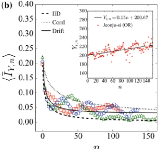
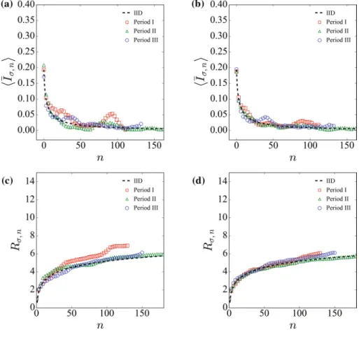
In Fig. 2 the moving average of ⟨IY,n⟩ over m = 18 steps (or 6 months) is applied to reduce noise [48]. The moving average, ⟨̄IY,n⟩ , is defined as
The obtained ⟨̄IY,n⟩ ’s for each regional group and period are shown in Fig. 2. For comparison, the analytic expressions of ⟨̄IY,n⟩ in Table 2 are also displayed in Fig. 2. In Fig. 2a we show ⟨̄IY,n⟩ ’s for OR. For period I, ⟨̄IY,n⟩ decreases when n ≳30 , then increases rapidly for 30 ≤ n ≤ 75 and decreases again for n ≥ 75 . Such rapid increases and decreases for n ≤75 might be an effect of the subprime mortgage crisis in the US. During the subprime mortgage crisis, the average (5)
⟨̄IY,n⟩ = 1 m
�m
k=0
⟨IY,n+k⟩.
Table 2 Summary of ⟨In⟩ and Rn for various sequence {xn} for n ≫ 1
𝜂n is the IID random variable drawn from symmetric and continuous distribution f(x). c is a constant repre- senting a constant drift, and 𝛾E is the Euler constant
Sequence xn ⟨In⟩ Rn Refs.
IID xn= 𝜂n 1
n
ln(n) + 𝛾E [1]
IID with drift xn= 𝜂n+ cn (c = const.) 1
n+ c2
√𝜋 e2
� ln(n2
8𝜋) ∑n
i=1 1 n+ c2
√𝜋 e2
� ln(n2
8𝜋) [2]
Correlated sequence xn= xn−1+ 𝜂n 1
√𝜋n
√2 𝜋
√n [3]
Fig. 2 Plots of a ⟨̄IY,n⟩ for OR and b for NR. Red squares represent period I, green triangles denote period II, and blue circles corre- spond to period III. The dashed line denotes the 1/n which corre- sponds to the ⟨̄In⟩ for IID sequence. The dotted line denotes the 1∕√
𝜋n which corresponds to the ⟨̄In⟩ for correlated sequence. The
solid lines represent a the relation ⟨̄IY,n⟩ = a cos(bn + c) + d with a= 0.05, b = 0.055, c = 𝜋∕2, d = 0.105 , and b 1n+ c2
√𝜋 e2
� ln(n2
8𝜋) with c = 0.018 . Inset: Yn against n. The solid line denotes Eq. (7).
From the best fit of the data to Eq. (7), we obtain ai≃ 0.15
value of Korea composite stock price index (KOSPI) sharply decreases, which causes the movement of speculative capi- tal from the stock market to the real estate market [49]. As a result, the price of house sharply increases after sudden decreases caused by the indirect effect of subprime mort- gage crisis in the US [50]. However, the behavior of ⟨̄IY,n⟩ for period I seems to be well described by the correlated sequence on the average, i.e., ⟨̄IY,n⟩ = 1∕√
𝜋n . On the other hand, the behavior of ⟨̄IY,n⟩ during period II for OR is well fitted to 1/n. This clearly shows that the change of price in period II is a simple random process (see Table 2), and agrees with the behavior of {Yn} for the period (see Fig. 1a, b). ⟨̄IY,n⟩ for period III is eccentric. ⟨̄IY,n⟩ in this period shows strong periodicity. Thus, we fit the data to the periodic func- tion as
From the best fit of the data to Eq. (6), we obtained A = 0.05 , B= 0.055 , 𝜙 = 𝜋∕2 , and I0= 0.105 . The obtained value of B = 0.055 means that the cycle of ⟨̄IY,n⟩ is repeated by n= 36 , which corresponds to 1 year exactly. Thus the peri- odic behavior of ⟨̄IY,n⟩ comes from the seasonal effect which agrees with the fact that the people prefer to move from spring to early summer in Korea. Thus, for spring and sum- mer the price increases rapidly and the record occurs more frequently than fall and winter.
In Fig. 2b we shows the behavior of ⟨̄IY,n⟩ ’s for NR. The data clearly show that all ⟨̄IY,n⟩ ’s for NR fluctuate between 1/n and 1∕√
𝜋n and the fluctuations of ⟨̄IY,n⟩ are significantly smaller than that for OR. For period I, ⟨̄IY,n⟩ decreases for n ≤40 , then slightly increases when the subprime mortgage crisis occurs ( 40 < n < 100 ). For n > 55 , ⟨̄IY,n⟩ seems to be well fitted by ⟨In⟩ = 1∕√
𝜋n . For period II, ⟨̄IY,n⟩ has a hump in the interval 20 < n < 80 . However, ⟨̄IY,n⟩ decreases as 1/n when n > 80 . During period III, ⟨̄IY,n⟩ also shows the perio- dicity with decaying amplitude and increasing period. Thus, we expect that the periodicity is not strong as for the same period in OR.
(6)
⟨̄IY,n⟩ = A cos(Bn𝜋 + 𝜙) + I0.
Since the values of ⟨̄IY,n⟩ for NR are bounded by 1/n and 1∕√
𝜋n , we can not exclude the possibility that the sequence of {Yi,n} can be described by IID with drift [4].
The drift constant c of the sequence is measured as follows [4]. As an example, {Yi,n} for i = [Jeonju district] in NR is shown in inset of Fig. 2b. We fit the {Yi,n} to the linear equation [4],
Here, ai and bi are fitting parameters for district i, and ai cor- responds to the drift constant [4] and 𝜖i represents an error.
In addition, we also measure the standard deviation si=
�∑
N
k=1(Yi,k−⟨Yi⟩)
N−1 for {Yi,n} . The normalized drift constant c is defined as [4]
From {Yi,n} for NR, we obtain c ≃ 0.018 for period III. The
⟨̄IY,n⟩ = 1n+ c2
√𝜋 e2
� ln(n2
8𝜋) for IID with drift constant c= 0.018 is shown in Fig. 2b. Therefore, the data for NR are also well described by the IID with constant drift on the average. The results obtained from Fig. 2a, b show that if the market is overheated then ⟨̄IY,n⟩ significantly deviates from the behavior of ⟨In⟩ for a sequence listed in Table 2, while
⟨̄IY,n⟩ is bounded between 1/n and 1∕√
𝜋n when the market is not overheated. Therefore, ⟨̄IY,n⟩ can be used as a simple proxy to measure the trading pattern in given districts.
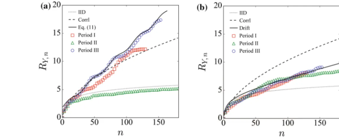
By using Eq. (4), we calculate the number of records up to nth steps, RY,n . In Fig. 3a we show the obtained RY,n
for each period in OR. Rn ’s in Table 2 are also displayed.
For period I in OR, we find that RY,n is well described by Rn of correlated sequence, Rn= 2𝜋√
n , as expected from Fig. 2a. For period II, RY,n is well described by ln(n) + 𝛾E
which corresponds to the RY,n for IID (see Table 2). From Eqs. (4, 6), RY,n for period III is obtained as
(7) Yi,n= ain+ bi+ 𝜖i.
(8) c= 1
D
∑D
i=1
ai si.
Fig. 3 Plots of a RY(t) for OR and b for NR. Red squares represent period I, green triangles denote period II, and blue circles correspond to period III. The dotted lines denote the ln(n) + 𝛾E for Rn of IID sequence, where 𝛾E is the Euler constant. The dashed line denote √2𝜋√
n for Rn of correlated sequence. The solid lines represent a Eq. (9) and b Eq. (10)
with A = 0.05 , B = 0.055 , 𝜙 = 𝜋∕2 , and I0= 0.105 . As shown in Fig. 3a, RY,n for period III is well described by Eq. (9). Since I0 is the most dominant term in Eq. (9) for sufficiently large n, RY,n grows almost linearly as n becomes large. This shows that RY,n grows linearly for extreme bull markets. In Fig. 3b, we display RY,n ’s for NR. The data clearly show that RY,n for all period significantly deviates from RY,n= ln n + 𝛾E and RY,n= 2√
n∕𝜋 . This means that {Yi,n} ’s for NR cannot be approximated by IID sequence and correlated sequence. In NR, we obtain c = 0.021 ± 0.003 for period I, c = 0.018 ± 0.002 for period II, and c= 0.018 ± 0.002 for period III from the data in Fig. 2. For all periods the obtained values of c coincide within the esti- mated errors. The solid line in Fig. 3b represents
(9) RY,n=
∑n
n�=1
[Acos(Bn�𝜋+ 𝜙) + I0] .
(10) Rn,c=
�n
k=1
1 k+ c2√
𝜋 e2
� ln
�k2 8𝜋
� ,
with c = 0.018 . As shown in Fig. 3b, Eq. (10) with c = 0.018 well describes the behaviors of RY,n for all periods. From these results, we find that the sequence of price in NR is most suitably described by the IID with a constant drift. This agrees with observed behavior of ⟨Y(n)⟩ for NR in Fig. 1c.
We also applied the same method to obtain ⟨̄I𝜎,n⟩ and R𝜎,n
for volatility sequence {𝜎i,n} . In Fig. 4, we plot the obtained
⟨̄I𝜎,n⟩ and R𝜎,n with theoretical expectations of ⟨̄I𝜎,n⟩ listed in Table 2. From the data in Fig. 4a, b, we find that ⟨̄I𝜎,n⟩ is well fitted to ⟨In⟩ = 1∕n . This implies that {𝜎i,n} is simply approxi- mated by IID sequence for all regions and periods. ⟨̄I𝜎,n⟩ for period I deviates from 1/n when 80 ≤ n ≤ 110 . By comparing with Fig. 2a, we expect that the deviation might be originated from subprime mortgage crisis in the US. R𝜎,n ’s for OR and NR are shown in Fig. 4c, d, respectively. In Fig. 4c, we find that R𝜎,n is well described by theoretically expected Rn for IID sequence except period I due to the effect of subprime mort- gage crisis. We also find that R𝜎,n for NR are identical with Rn
for IID sequence. Therefore, R𝜎,n and ⟨̄I𝜎,n⟩ seem to be hardly affected by exogenous financial factors in contrast to the RY,n
and ⟨̄IY,n⟩.
Fig. 4 Plots of a ⟨̄I𝜎,n⟩ for OR, b for NR and c R𝜎,n for OR, d for NR. Red squares represent period I, green triangles denote period II, and blue circle cor- respond to the period III. In a and b, the dashed lines denotes the 1/n for ⟨̄In⟩ obtained from IID sequence. In (c) and (d), The dashed lines denotes the ln(n) + 𝛾E
5 Conclusion
We numerically analyze the behaviors of the record statistics of apartment prices in the Korean housing market for the period 1 Jan. 2006 to 31 Dec. 2018. We divide the market into two groups, OR and NR, based on the trading pattern.
We also divided the given time series into three distinctive periods based on the behavior of price. From the measure- ment of record rate and expected number of records in the transaction data of the Korean housing market, we find different patterns for price and volatility sequence in each regional group and period. The record rate of price, ⟨̄IY,n⟩ , in OR behaves like a correlated sequence for period I, during which the Korean housing market is strongly affected by the subprime mortgage crisis in the US. On the other hand, for period II in OR, ⟨̄IY,n⟩ agrees very well with that for IID random sequence. The more interesting finding is that ⟨̄IY,n⟩ shows a strong seasonal effect for period III. For period III the price of an apartment in Korea continuously increases.
Thus the market is regarded as a bull market for period III.
On the other hand, ⟨̄IY,n⟩ and the expected number of record for the price, RY,n , in NR show that the record statistics is well approximated by the IID random sequence with drift. In contrast to the behaviors of ⟨̄IY,n⟩ and RY,n , ⟨̄I𝜎,n⟩ and R𝜎,n do not show any characteristic feature. This clearly shows that both ⟨̄IY,n⟩ and RY,n are good proxy to understand the market dynamics rather than ⟨̄I𝜎,n⟩ and R𝜎,n.
As a final remark, we also investigate the record statistics for logarithmic return, 𝜌i(n) , defined in Eq. (1). However, we find that the change in 𝜌i(n) was not much different from the results obtained from volatility. In addition, we also test the effect of inflation on the house prices record statistics in Korea. Since the inflation rate in Korea is relatively small than the increment of house prices, we find that the statisti- cal properties of records for house prices are not affected by the inflation.
Acknowledgements This research was supported by Basic Science Research Program through the National Research Foundation of Korea (NRF) funded by the Ministry of Education (Republic of Korea) (Grant number: NRF-2019R1F1A1058549).
References
1. J. Krug, J. Stat. Mech.: Theory E. 2007, P07001 (2007) 2. J. Franke, G. Wergen, J. Krug, J. Stat. Mech.: Theory E. 2010,
P10013 (2010)
3. S.N. Majumdar, R.M. Ziff, Phys. Rev. Lett. 101, 050601 (2008) 4. G. Wergen, M. Bogner, J. Krug, Phys. Rev. E 83, 051109 (2011) 5. C. Godreche, S.N. Majumdar, G. Schehr, J. Phys. A: Math. Theor.
50, 333001 (2017)
6. G. Wergen, S.N. Majumdar, G. Schehr, Phys. Rev. E 86, 011119 (2012)
7. E.J. Gumbel, Statistics of Extremes (Dover, New York, 1958).
8. N.C. Matalas, Clim. Change 37, 89 (1997)
9. S. Redner, M.R. Petersen, Phys. Rev. E 74, 061114 (2006) 10. A. Anderson, A. Kostinski, J. Appl. Meteorol. Clim. 50, 1859
(2011)
11. J. Krug, K. Jain, Physica A 358, 1 (2005) 12. N. Glick, Am. Math. Mon. 85, 2 (1978)
13. E. Ben-Naim, S. Redner, F. Vazquez, Europhys. Lett. 77, 30005 (2007)
14. G. Wergen, Physica A 396, 114 (2014)
15. P. Joyce, D.R. Rokyta, C.J. Beisel, H.A. Orr, Genetics 180, 1627 (2008)
16. D.R. Rokyta et al., J. Mol. Evol. 67, 368 (2008)
17. Y. Edery, A.B. Kostinski, S.N. Majumdar, B. Berkowitz, Phys.
Rev. Lett. 110, 180602 (2013)
18. S.N. Majumdar, P. von Bomhard, J. Krug, Phys. Rev. Lett. 122, 158702 (2019)
19. G. Wergen, J. Krug, Europhys. Lett. 92, 30008 (2010)
20. M. Karsai, K. Kaski, A.-L. Barabási, J. Kertész, Sci. Rep. 2, 1 (2012)
21. R.N. Mantegna, H.E. Stanley, Introduction to Econophysics:
Correlations and Complexity in Finance (Cambridge University Press, Cambridge, 1999).
22. J.-P. Bouchaud, M. Potters, Theory of Financial Risk and Deriva- tive Pricing: From Statistical Physics to Risk Management (Cam- bridge University Press, Cambridge, 2003).
23. V. Plerou et al., Phys. Rev. E 60, 6519 (1999)
24. X. Gabaix, P. Gopikrishnan, V. Plerou, H.E. Stanley, Nature 423, 267 (2003)
25. R.N. Mantegna, H.E. Stanley, Nature 376, 46 (1995) 26. U.A. Müller et al., J. Bank. Finance 14, 1189 (1990) 27. Y. Liu et al., Phys. Rev. E 60, 1390 (1999)
28. P. Cizeau et al., Physica A 245, 441 (1997)
29. D. Sornette, Why Stock Markets Crash: Critical Events in Com- plex Financial Systems, vol. 49 (Princeton University Press, Princeton, 2017).
30. F.M. Longin, J. Bus 69, 383–408 (1996)
31. A. Johansen, D. Sornette, Eur. Phys. J. B 1, 141 (1998) 32. M.B. Roehner, Evol. Inst. Econ. Rev. 2, 167 (2006) 33. P. Richmond, Physica A 375, 281 (2007)
34. P. Richmond, B. Roehner, Evol. Inst. Econ. Rev. 9, 125 (2012) 35. C.R. Cunningham, J. Urban Econ. 59, 1 (2006)
36. Z. Adams, R. Füss, J. Hous. Econ. 19, 38 (2010)
37. J. Aizenman, Y. Jinjarak, H. Zheng, VoxEU. org 24 (2016) 38. G. Meen, J. Hous. Econ. 11, 1 (2002)
39. J. Kim, J. Park, J. Choi, S.-H. Yook, J. Korean Phys. Soc. 73, 1431 (2018)
40. https ://www.data.go.kr. Accessed 8 Sept 2020 41. https ://elaw.klri.re.kr. Accessed 8 Sept 2020 42. http://www.kosis .kr. Accessed 8 Sept 2020 43. http://stat.molit .go.kr. Accessed 8 Sept 2020
44. T.G. Andersen, R.A. Davis, J.-P. Kreiß, T.V. Mikosch, Handbook of Financial Time Series (Springer Science & Business Media, Berlin, 2009).
45. Z. Zheng et al., PLoS ONE 9, e102940 (2014) 46. S.J. Taylor, B. Letham, Am. Stat. 72, 37 (2018) 47. S. Kumar, N. Deo, Phys. Rev. E 86, 026101 (2012)
48. S.W. Smith, The Scientist and Engineer’s Guide to Digital Signal Processing (California Technical Pub, San Diego, 1997).
49. J.R. Kim, G. Lim, Econ. Model. 59, 174 (2016) 50. J. Chang, SERI Q. 2, 25 (2009)
Publisher’s Note Springer Nature remains neutral with regard to jurisdictional claims in published maps and institutional affiliations.