ICCAS2005ICCAS2005 June 2-5, KINTEX, Gyeonggi-Do, Korea
1. INTRODUCTION
In an autonomous vehicle, position sensing is an important task for the identification of vehicle’s locations, such as the lateral position relative to a lane or a desired trajectory. Technologies developed for identifying the vehicle’s location include electrically powered wire, computer vision, magnetic sensing, optical sensing, inertia navigation, and global positioning systems [1,3]. This paper focus on magnetic sensing systems[4-7] that are used for ground vehicle control and guidance.
The magnetic marking scheme has several advantages compared with the electrified wiring scheme. Since it is a passive system, it is simple and does not use any energy. A vision sensing scheme is expensive to acquire and to process the optical images into credible data in real-time in any weather and road conditions. In the positioning reference system, magnets are embedded just under the surface of a road as Figure 1 shows. The magnetic fields generated by these magnets are detected by magnetic sensor mounted under the bumpers of the test vehicle.
Fig. 1 Position sensing using magnetic sensor and magnets. The major concern in implementing a magnetic sensing system on roads is the background magnetic field. For magnetic sensing, it is a problem that the magnitude of the background magnetic field is not small compared to that of the magnet’s magnetic field. The background field may be stable or varying, depending on the specific location or the orientation.
This paper suggests a design of the position sensing system
and discusses the related technical issues. In this paper, the position sensing technique is first illustrated in
Section 2 by introducing the magnetic patterns produced by a sample magnet. The analysis and measurement system for magnetic field in Section 3. The paper concludes with a discussion of these concerns in Section 4.
Analysis of Magnetic Marker for Autonomous Vehicle Guidance System
Using 3-axis Magnetic Sensor
Dae-Young Lim*, Young-Jae Ryoo*, Eui-Sun Kim**, Jei-Kyun Mok***
*
Department of Control System Engineering, Mokpo National University, Jeonnam, Korea(Tel : +82-61-450-2754; E-mail: [email protected]) (Tel : +82-61-450-2754; E-mail: [email protected])
**
Department of Electrical &Electronics Engineering, Seonam University, Jeonbok, Korea (Tel : +82 -063-620-0249; E-mail: [email protected])***
New-energy Urban Train Team, Korea Railroad Research Institute, Kyounggi, Korea (Tel : +82-031-460-5727; E-mail: jkmok @krri.re.kr)Abstract: In this paper, analysis of magnetic marker for autonomous vehicle guidance system using 3-axis magnetic sensor propose. Position sensing is an important an estimation system of vehicle position and orientation on magnetic lane, which is a parameter of the steering controller for automated lane following is described. To verify that the magnetic dipole model could be applied to a magnetic unit paved in roadway, the analysis of the data 3-axis magnetic field measured experimentally.
Keywords: Autonomous vehicle, Magnetic marker, Magnetic sensor, Position sensing.
2. MAGNETIC FIELD OF MAGNET
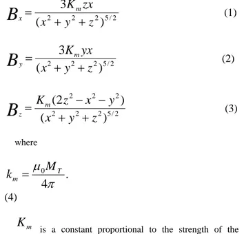
In this section, the comprehensive analysis of the magnetic field of a magnet used for position sensing is presented. Since a typical magnet has the shape of a cylindrical permanent magnet, assume that the magnet is a magnetic dipole. The magnetic field around a magnet can be described using rectangular coordinates as (see Figure 2) [8].2 / 5 2 2 2
)
(
3
z
y
x
zx
K
m xB
=
+
+
(1)
2 / 5 2 2 2)
(
3
z
y
x
yx
K
m yB
=
+
+
(2)
2 / 5 2 2 2 2 2 2)
(
)
2
(
z
y
x
y
x
z
K
m zB
=
+
−
+
−
(3)
where.
4
0π
µ
T mM
k
=
mK
0 2M
b
M
T=
π
(4)
is a constant proportional to the strength of the magnet.
(5)
ICCAS2005 June 2-5, KINTEX, Gyeonggi-Do, Korea
where is the magnetization surface charge density,
and is the radius of the cylindrical permanent magnet.
0
M
b
Fig. 2 Magnetic field of magnet.
Figure 2 depicts the three-axis components of the magnetic field using rectangular coordinates. The longitudinal component is parallel to the line of magnet installation on the road, the vertical component perpendicular to the surface, and the lateral component perpendicular to the other two axes. The longitudinal, the lateral, and the vertical component of the magnetic field can be transformed from the polar coordinate equations as:
) (Bx
)
(
B
z)
(
B
y ) m K( x
)
)
( y
( z
)
As(1), (2) and (3) show, each component of the field is a function of the strength ( , the longitudinal , the lateral , and the vertical distance to the sensor.
3. ANALYSIS AND MEASURE MENT SYSTEM
FOR MAGNETIC FIELD
Fig. 3 Magnetic field measurement system.
Figure 3 shows the magnetic fields measuring system. The sample marker is ferrite magnet in a cylindrical shape with a diameter of size 2.5cm and length of 10cm, neodymium diameter of size 2.5cm and length of 8cm. The axis of the cylinder is placed perpendicular to the surface of the bench table. The measurements took place with a magnetic sensor at several different heights from the surface of the table to acquire a representative map of the magnetic field. For illustration, the data with the sensor at 20cm height is shown in Figure4, 5, and 6.
The sensor is a Honeywell HMR2300. These sensor is a three-axis smart digital magnetometer to detect the strength and direction of an incident magnetic field. The three of magneto-resistive sensors are oriented in orthogonal directions to measure the X, Y and Z vector components of a magnetic field. These sensor outputs are converted to 16-bit digital values using an internal A/D converter. An onboard EEPROM stores the magnetometer’s configuration for consistent operation. The data output is serial full-duplex RS-232 with 9,600 or 19,200 data rates. The range is 2 Gauss, <70ugauss Resolution.
To verify that these model equations of (1), (2) and (3) represent the physical magnetic fields, the equations are compared with the direct experimental measurement using a ruler on the x-y test bench table. Test bench is size of 100*100[cm]. The magnetic sensor was mounted in a plane above 30[cm] from the upper end of the magnet.
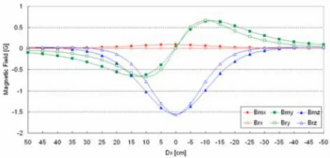
Fig. 4. Comparison of the model equations with the direct measurement using a ruler.
Figure 4 shows the comparison of the magnetic field
components calculated by the magnetic model equations with those measured by the experiment at various distances to the magnet. The data shows that these model equations are very accurate with the maximum error of only 92mG along longitudinal , and 260mG along vertical magnetic vertical magnetic field . Thus, the assumption of a dipole magnet is reasonable, and the model equations are useful to represent the magnetic field.) (Bx ) (Bz ) (Bx
)
yB
3.1 Distribution magnetic field of magnetic markerIn figure 4 the longitudinal component rise from zero at the center of the magnet and reaches its peak at a distance about 100mm from the magnet, then gradually weakens farther away from the magnet. The peak value for this data set is about -1.1mG, 210mG. The longitudinal field makes a steep transition near the magnet as it changes its sign. This steep transition becomes meaningful in interpreting the point at which a sensor passes over a magnet location
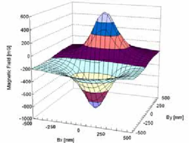
As shown in Figure 5 the lateral component
(
reaches its peak at the top of the magnet, and drops down to zero at about 500mm away from the magnet. The peak valueICCAS2005 June 2-5, KINTEX, Gyeonggi-Do, Korea
for the data set of lateral component is about 990mG, 410mG.
In any horizontal plane parallel to that of the magnet, as a function of distance from the magnet, the patterns of
and measurements are similar.
x
B
B
yFig. 4 Longitudinal component of magnetic field of a magnet with sensor at 10cm high.
Fig. 5 Lateral component of magnetic field of a magnet with sensor at 10cm high.
Fig. 6 Vertical component of magnetic field of a magnet with sensor at 10cm high.
In Figure 6, the vertical field is the strongest right at the top of the magnet, and diminishes to zero at about 500mm away from the magnet. The peak value is above 1420mG. The vertical field quickly drops as it moves away from the magnet. Since the vertical field is the strongest component among the measurements near the magnet, its use will be significant is identifying the closeness of a magnet.
)
(
B
z3.2 Comparisons of magnetic field from different markers
Fig. 7 Comparisons of ferrite and neodymium marker. Figure 7 shows the comparisons of a ferrite and neodymium marker measured at a sensor height of 10cm. The dotted line is neodymium magnet but solid line is ferrite magnet. Therefore seen the neodymium bigger than ferrite.
3.3 Position sensing from magnetic fields
Once the magnetic fields are measured, the measured fields at that location will be used to identify the distance to the magnet.
From(5), (6) and (7), the sensor position can e derived as:
)
,
(
x
y
3 / 1 2 / 5 2 2 2 3)
6
18
24
24
(
256
)
3
(
3
⎪⎭
⎪
⎬
⎫
⎪⎩
⎪
⎨
⎧
+
+
+
+
=
C
B
B
B
B
B
C
B
k
x
z z y x x z m(6)
x
B
B
y
x y=
(7)
Where ±+
+
=
2 2 29
8
8
B
xB
yB
zC
. (8)
According to equations (6), (7), and (8), the position of the sensor with respect to the magnets can be calculated. The inverse mapping equations are useful to estimate the position continuously as long as the magnetic field is strong enough to be sensed. In the implemented system, the transformation of the measured signals to the distance to the magnet is based on the inverse mapping relationship.
4. CONCLUSION
In this paper, analysis of magnetic marker for autonomous
vehicle guidance system using 3-axis magnetic sensor propose. Position sensing is an important an estimation system of vehicle position and orientation on magnetic lane, which is aICCAS2005 June 2-5, KINTEX, Gyeonggi-Do, Korea
parameter of the steering controller for automated lane
following is described. To verify that the magnetic dipole model could be applied to a magnetic unit paved in roadway, the analysis of the data 3-axis magnetic field measured experimentally.
ACKNOWLEDGMENTS
This paper was supported by “National Transportation Key Technology R&D Project”
REFERENCES
[1] Y. J. Ryoo and Y. C Lim, “Coordinated Control of Speed and Steering System Based on Neural Network for Automated Lane Following Vehicle,” International
Conference on Electrical Engineering 1999, Vol. 1, pp.
370-373, 1999.
[2] K. M. Passio, “Intelligent control for autonomous vehicle,” IEEE Spectrum, pp. 55-62, 1995.
[3] Y. J. Ryoo and Y. C. Lim, “Visual control of autonomous vehicle by neural networks using fuzzy-supervised learning,” Journal of electrical
engineering and information science, Vol.2, no.2,
pp.77-85, 1997.
[4] C. Y. Chan and H. T. Tan, “Evaluation of Magnetic as a Position Reference System For Ground Vehicle Guidance and Control,” California Path Research
Report, UCB-ITS-RRR-2003-8, March, 2003.
[5] C. Y. Chan, “A System Review of Magnetic Sensing System for Ground Vehicle Control and Guidance,”
California PATH Research Report.
UCB-ITS-PRR-2002-20 May, 2002.
[6] C. Y. Chan, “Magnetic sensing as a position reference system for ground vehicle control,” IEEE Trans. Inst.
and Meas., vol.51, no.1, pp.43-52, Dec. 2002.
[7] H. S. Tan, J. Guldner, S. Patwardhan, C. Chen, and B. Bougler, “Development of an automated steering vehicle based on road magnets –a case study of mechatronic system design”, IEE/ASME Transactions on Mecartonics, Vol. 4, no. 3, pp.258-272, Sept. 1999.
[8] E. S. shire, Classical electricity and magnetism, Cambridge, U.K Cambridge University Press, 1960.