46-4 / J. J. Jensen
IMID 2009 DIGEST •
Abstract
This paper reports of camera detection of Mura. The type, location, size, orientation and amplitude are found. As the luminance variation in Mura is down to less than app. 0.3 %, measurement apparatus, techniques and algorithms are developed to measure low noise data and to extract the Mura from data with the residual noise in the same magnitude as the Mura.
1.
Introduction
One of the most important quality parameters for a FPD is the level of Mura, and today this level is found by (well trained) humans. The Mura is estimated at low luminance levels as it seems that the Mura defects are most visible at a luminance level below 50 cd/m2, down to say 5 cd/m2 and even lower. Typically each display must be evaluated in less than 30 sec, due to the speed of the production line.
The Mura is detected as a subtle change in luminance over an area of the FPD. The shape of the area can be like points, lines, band and spots. The change of luminance can be as low as 0.3 % of the average luminance level. An instrument for Mura detection must give both spatial and luminance information of the FPD under test. The only types of Light Measuring Device (LMD) that can do that are 2D luminance cameras.
The 2D luminance camera must be able to do a measurement at low luminance level with a noise level preferable lower than the change in luminance in the Mura, with a spatial resolution comparable to the pixel size of the FPD and even do the measurement (and analyze of the data) within the period allowed by the speed of the production line.
Given the CCD, the noise level will depend on the square root of the number of electrons captured in the camera pixels. Quad doubling the number of collected
electrons will half the noise. To collect many electrons the ‘light’ sensitivity of the 2D luminance camera has to be high and the CCD must have a well size big enough to hold the electrons. As the well size is proportional to surface area of the pixel it can be a trade-off with the resolution. But in the end the most important is not the well size or the number of bits in the AD converter; it is simply how many electrons can be collected in a given period of time.
2. Experimental
Several FPD were measured with the 2D camera ICAM, from DELTA, Denmark.
Example 1: In fig. 1 it is possible to see an erroneous application of liquid crystal. In fig. 2 the luminance distribution of the raw data is shown (as a red curve) along the line indicated in figure 1. A Mura with this magnitude (app. ±1%) is easily found, but the example is used to discuss the limits for robust detection.
The standard deviation in the high frequency noise is found to 0.144 cd/m2 at an average luminance level
of 112.1 cd/m2. We define the limit of detection
(LOD) as 3 times the standard deviation of the noise. This indicates that a change in luminance in just one ICAM pixel on 0.433 cd/m2 (0.39 % of the average luminance level) will be detectable. The data is ‘cleaned’ for the high frequency (HF) noise and the low frequency (LF) noise. This is show as a black curve in fig. 2For the majority of Mura types it will be possible to utilize some kind of intelligent averaging and hereby push the detection limit further down.
It is a simple matter to automatically detect the presence, amplitude and orientation of this Mura.
Luminance measurement at low levels for detecting Mura
Jens Joergen Jensen1, René Bolvig Stentebjerg2 and Jack Frausing2
1DELTA, Light & Optics, Hoersholm, Denmark Tel.:+45 72194000, E-mail: [email protected] 2DELTA, Light & Optics, Hoersholm, Denmark
46-4 / J. J. Jensen
• IMID 2009 DIGEST
Fig. 1. Same LCD TV with luminance level shown in false color. Detection of Mura 105 110 115 120 0 100 200 300 400 500 600 700 800 900 Pixel Lu mi na nc e Measurement LF and HF removed
Fig. 2. Measurement and data, where HF and LF are removed, for Mura detection
Example 2: In figure 3 top-left is show the luminance variation on an LCD where the LC is dispensed by a one drop fill dispenser.
The average luminance of the display is app. 3.5 cd/m2 and the luminance variations we want to detect
is app. ±1.5%. The difficult part in this measurement is to measure a small absolute difference in luminance, at a very low luminance level and do it within a few seconds. Here less than 5 sec. was enough to do a measurement where the noise level in the raw data was app. 0.7%. The result of the measurement and data manipulation is shown in the 4 images in fig. 3. Top-left shows the raw data, top right shows the calculated LF component, bottom-left show data with the LF removed and the bottom-right shows this data smoothed. See also fig.4.
Fig. 3. One drop filled LCD panel. Top-left: raw luminance data. Top-right. The calculated LF component. left. Data without LF. Bottom-right. Data without LF and HF.
DataG
Fig. 4. Data without LF and HF.
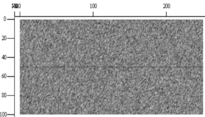
Example 3: Simulated Line Mura. In figure 5 is shown a simulated part of a display with a line Mura. Size is 251 x 101 pixels and the background luminance is 100.0 cd/m2 with σ=0.20 cd/m2. The Line Mura is 1
pixel wide and the luminance is 99.4 cd/m2 with
46-4 / J. J. Jensen
IMID 2009 DIGEST •
the Line Mura is shown. The only value that is just more than 3 times σ lower than the average is right at the Line Mura position. In figure 7, the profile is found by averaging over 3 columns. It is likely that a point Mura can be detected, while a line Mura of length 3 most certainly will be detected.
Fig. 5. Simulated Line Mura. Level is 100 cd/m2 and noise level 0.2 cd/m2.
0 20 40 60 80 100 99.5 100 100.5 Ave−3 Std⋅ Ave
Fig. 6. Pixel data with noise 0.2 cd/m2.
0 20 40 60 80 100 99.5 100 100.5 Ave −3 Std⋅ Ave
Fig. 7. noise 0.2 cd/m2. Average over 3 columns.
If we increase the noise of the background luminance (measured pixel values) to the same amount as the Mura contrast, σ=0.60 cd/m2 we cannot detect a single
point but only a longer line. See fig. 8. In fig. 9 the luminance profile is shown. It is seen that detection is impossible. The minimum length of the line, that can be detected, can be calculated as:
2 ⎟ ⎠ ⎞ ⎜ ⎝ ⎛ = st MuraContra LOD Length
By averaging 9 columns the line Mura becomes
detectable, but the resolution on the line Mura length is lower. Se figure 10.
Fig. 8. Simulated Line Mura. Level is 100 cd/m2 and noise level 0.6 cd/m2.
0 20 40 60 80 100
100 102
Ave −3 Std⋅ Ave
Fig. 9. Pixel data with noise 0.6 cd/m2.
0 20 40 60 80 100 99.5 100 100.5 Ave −3 Std⋅ Ave
Fig. 10. Pixel data with noise 0.6 cd/m2. Average over 9 columns.
So if the noise increases, the size of a detectable Mura increases. If the noise can be reduced by averaging more and more pixels (larger Mura’s) even a small contrast Mura can be found in very noisy data, but with the cost of a lower Mura resolution. The number of pixel is limited and therefore the precision must have a certain level. Further some noise in the data cannot be removed.
In figure 10 is added a slowly variation in the background luminance (as from the BLU). The amplitude of this variation, 0.6 cd/m2, adds to standard
46-4 / J. J. Jensen
• IMID 2009 DIGEST
deviation and hereby the difficulty of finding the line Mura increases. In figure 11 the luminance profile for an average of 9 columns is shown while in figure 12, the luminance profile for an average of 61 columns is shown.
Fig. 10. Simulated Line Mura. Level is 100 cd/m2, noise level 0.6 cd/m2 and LF background variation is 0.6 cd/m2 0 20 40 60 80 100 99 100 101 Ave −3 Std⋅ Ave
Fig. 11. Level is 100 cd/m2, noise level 0.6 cd/m2 and LF background variation is 0.6 cd/m2. Average over 9 columns. 0 20 40 60 80 100 99 100 101 Ave −3 Std⋅ Ave
Fig. 12. Level is 100 cd/m2, noise level 0.6 cd/m2 and LF background variation is 0.6 cd/m2. Average over 61 columns.
It is seen that averaging do not reduce the overall LOD, but only the local. The luminance profile does still have the variation but is found with less noise. To find Mura’s in this kind of data, involves more sophisticated algorithms, but depending on the nature and amplitude of this variation it might be impossible.
3. Results and discussion
It is shown that Mura can always be detected if the noise in the data given as the standard deviation is less than app. 1/3 of the Mura level to be found. If there is a slowly variation in the background luminance (BLU etc.), it impossible to do a robust detection. This variation can be removed and maybe characterized as a kind of Mura.
If the Mura has certain geometries (line, band, circle, etc) it is possible to do intelligent averaging without destroying the shape and size of the Mura. The disadvantage is that the Mura must be of a minimum size.
The possibility to measure and automatically quantify Mura on-line will give the industry access to high quality and repeatable data that can be used for feed back to the production line, better sorting and thereby a more uniform quality; and a quality agreed on by both producer and costumer.
Acknowledgement
This work was funded by DELTA Light & Optics, Denmark
5. References
1. 5725 – 1:1994, Accuracy (trueness and precision) of measurement methods and results. Part 1: General ISO principles and definitions.