752
-Destripe Hyperspectral Images with Spectral-spatial Adaptive Unidirectional
Variation and Sparse Representation
Dabiao Zhou1,2*, Dejiang Wang1, Lijun Huo2, and Ping Jia1
1Key Laboratory of Airborne Optical Imaging and Measurement, Changchun Institute of Optics, Fine
Mechanics and Physics, Chinese Academy of Sciences, Changchun 130033, China
2University of Chinese Academy of Sciences, Beijing 100049, China
(Received July 11, 2016 : revised November 28, 2016 : accepted November 29, 2016)
Hyperspectral images are often contaminated with stripe noise, which severely degrades the imaging quality and the precision of the subsequent processing. In this paper, a variational model is proposed by employing spectral-spatial adaptive unidirectional variation and a sparse representation. Unlike traditional methods, we exploit the spectral correction and remove stripes in different bands and different regions adaptively, instead of selecting parameters band by band. The regularization strength adapts to the spectrally varying stripe intensities and the spatially varying texture information. Spectral correlation is exploited via dictionary learning in the sparse representation framework to prevent spectral distortion. Moreover, the minimization problem, which contains two unsmooth and inseparable l1-norm terms, is optimized by the split Bregman approach. Experimental results, on datasets from several imaging systems, demonstrate that the proposed method can remove stripe noise effectively and adaptively, as well as preserve original detail information.
Keywords : Destriping, Total variation, Sparse representation, Hyperspectral images
OCIS codes : (100.2000) Digital image processing; (010.0280) Remote sensing and sensors; (100.3020) Image reconstruction-restoration
*Corresponding author: [email protected]
Color versions of one or more of the figures in this paper are available online.
*
This is an Open Access article distributed under the terms of the Creative Commons Attribution Non-Commercial License (http://creativecommons.org/ licenses/by-nc/3.0/) which permits unrestricted non-commercial use, distribution, and reproduction in any medium, provided the original work is properly cited.
*Copyright 2016 Optical Society of Korea
I. INTRODUCTION
Hyperspectral images (HSIs) have been successfully applied to a myriad of applications such as data classification and target detection [1]. However, they are inevitably contaminated with striping artifacts due to response variations of each detector. The existence of stripe noise not only degrades the image quality, but also limits the precision of the sub-sequent data analysis. Consub-sequently, it is an essential prepro-cessing step to remove the stripes.
In the past decades, several methods have been proposed in the extensive literature [2], and can be broadly classified into three major categories. The first category eliminates the striping pattern by filtering techniques. Filters in the spatial domain have the disadvantage of image information loss in spite of simple implementation [3]. Wavelet-based
filters only adjust the vertical or horizontal detail components [4-7]. Nonetheless, the structural information with the same frequency is unavoidably removed, which results in blurring and ringing artifacts. The second category, including histogram matching [8] and moment matching [9], makes use of similar statistics of individual detectors and restricts statistical parameters to a predefined reference. Though image statistical properties can be preserved, these equalization methods are highly sensitive to the assumption of statistical homogeneity. The third category is a variational approach [10-12]. The destriping issue is formulated as an inverse problem, and can be tackled in the regularization framework. Despite the effectiveness of these methods, the selection of regulation parameters has a great influence on the performance of destriping results [13].
spectrally varying stripes in HSIs. Even in the same band, stripe intensities may be spatially dependent. Thus, selecting regulation parameters band by band is particularly time-consuming and poses a challenging problem to conventional solutions. In Ref. [14], a spectral-spatial adaptive hypers-pectral total variation (SSAHTV) denoising model was proposed, in which the regulation parameters accommodated to the differences of the spectral noise and the spatial information. Nevertheless, the results for heavy stripes are not satisfactory, because this model fails to consider the unidirectional property of stripes.
Different from a single image, HSIs usually have hundreds of bands. Furthermore, high spectral correlation exists between adjacent bands. If the stripes are suppressed in the spatial domain only, spectral distortion will be introduced in the destriped image. However, little effort has been devoted to dealing with the spectral correlation. Recently, the sparse representation technique has been successfully applied in denoising problems [15-18]. It is based on the assumption that the noise-free image can be estimated by a linear combination of a few atoms in a redundant dictionary, which can be learned by utilizing the correlation and redundancy in an image [19].
Motivated by the success of the adaptive mechanism in SSAHTV model and the sparse representation in exploiting HSI correlation, we propose a unified spectral-spatial adaptive unidirectional variation and sparse representation method to counter the above problems. The proposed model consists of two l1-norm terms to stress the stripes adaptively, and an l2-norm term to handle the spectral correlations. The main ideas and contributions of the proposed approach are threefold as follows: i) Unidirectional variation and the spectral-spatial adaptive mechanism are combined to tackle the striping issue. Our method taps into the anisotropic characteristic of the stripes and the differences of spectral-spatial information simultaneously. ii) Spectral redundancy and correlation are exploited through a sparse representation prior imposed on the cost function to prevent spectral distortion. iii) The split Bregman algorithm is applied to solve and accelerate the model optimization, which is demonstrated to be remarkably effective and efficient.
This paper is organized as follows. In Section 2, we describe the spectral-spatial adaptive unidirectional variational model, the sparsity constraint, and the optimization process. Section 3 presents experimental results on synthetic and real images, and discusses the selection of optimal parameters. Finally, summarizations and conclusions are presented in Section 4.
II. METHODOLOGY
2.1 Problem Formulation
In this paper, the stripes are assumed to be additive, and the noisy HSI f can be modeled as
f = u + s (1)
where u is the noise-free HSI, and s is the vertical stripe noise. f ∈ RM×N×B is the noisy HSI. M and N refer to the height and width of the image, and B stands for the band number. Formally, the objective of HSI destriping is to retrieve u by removing s from f, which is a typical inverse problem and can be solved in the variational framework [20-23].
The stripes are highly anisotropic and have a directional property, which indicates that only the gradient perpendicular to the stripes is influenced. Motivated by this observation, the authors of Ref. [10] formulated an intuitive unidirectional variation (UV) model as
(
)
1 1minu x uj fj j yuj
j ∇ − +τ ∇ (2)
where ∇ and ∇ denoted vertical (i.e., x-coordinates) and horizontal (i.e., y-coordinates) derivative operators, respecti-vely. Here, j indexes the spectral channel. The UV model is comprised of a fidelity term to preserve the l1-norm of
the vertical gradient, and a regulation term to penalize the l1-norm of the horizontal gradient. The regulation parameter
τj determines the destriping strength.
The simplest way to destripe HSIs with the UV model is to handle each single band with possibly different τj.
However, selecting τj band by band manually is very
time-consuming, as HSIs have hundreds of bands. Therefore, a natural extension to a hyperspectral unidirectional variational (HUV) model is averaging out (2) with the same parameter τ for all the B bands,
(
)
[
]
∑
B= ∇ − + ∇ j x j j y j uj B 1 u f 1 u 1 1 min τ (3)Then, by taking partial derivatives of the cost function (3) with respect to uj, ∇, and ∇, we arrive at the
following Euler-Lagrange equation,
∇
∇ ∇
∇
∇ ∇
(4)where ⋅ represents the absolute value operator. Eq. (4) indicates that different bands are still considered as independent. That is, HSIs are destriped channel by channel, which has the following drawbacks. For different bands, large values of τ are prone to destroy fine features in the bands with slight stripes, and conversely, small values of τ may lead to incomplete removal of noise in the bands with severe stripes. For the same band, the stripes in flat regions will not be well suppressed if τ is too small, and detail information in the regions with abundant textures will be blurred if τ
is too large. Obviously, the parameter τ should be spectrally and spatially adaptive.
2.2. Spectral-spatial Adaptive Unidirectional Variation Model
To make the HUV model spectrally adaptive, we borrow the color total variation (CTV) model from Ref. [24] and redefine the HUV model as follows:
(
)
1( )
1 1 1 min u f R u B x j j y B j u∑
= ∇ − +τ ∇ (5) Here, ∇
∇
(6)introduces a coupling among all the spectral bands, where R( ․ ) is the root mean square (RMS) operator. A similar SSAHTV model for Gaussian noise was proposed previously in Ref. [9], where the TV model of each band was added together, without tapping into the directional characteristic of the stripes.
Similarly, the Euler-Lagrange equation derived from (5) takes the following form,
∇
∇ ∇
∇
∇ ∇ ⋅∇∇
(7) It is shown that a coupling term ∇∇ appears,and strikes a balance of the regularization strength between different bands. In essence, it is small for the bands with slight stripes, which turns down the regularization to preserve data genuineness. On the contrary, it is large for the bands with severe stripes, which emphasizes the regularization to entirely remove the stripes.
Besides the spectrally adaptive property discussed above, the spatially dependent property in different regions remains a critical problem. We use a simple spatial information extractor dj called difference curvature [24-26] to distinguish edges from ramps in the presence of noise,
(8)
Here, η corresponds to the gradient direction, and ε is the direction perpendicular to η . ujη η and ujεε are the second-order directional derivatives of uj, as defined in Ref. [27].
Then, we define a spatially adaptive weighting matrix W, whose elements are defined as
(9)
Here, µ is a positive constant, and ri is the i-th element of
R(d). Note that d = . For the pixels in the flat
areas, ri is small and Wi approaches 1, which leads to a large regularization strength to well suppress the stripes. Conversely, for the pixels corresponding to the structural details, ri is large and Wi approaches null, which weakens the regularization strength to preserve textures. The weighting matrix W is justified since it depends explicitly on the edge indicator, hence, it adapts implicitly to the spatial property.
Embedding the weight in Eq. (9) into Eq. (5), a novel spectral-spatial adaptive unidirectional variational (SSAUV) model is thus
(
)
1(
)
11
minu B ∇xu −f +τ WR∇yuj (10)
2.3. Sparse Representation Regulation
The above SSAUV model fails to take the spectral correlation into consideration. To tackle this problem, we merge the SSAUV model with a sparse representation, in which the spectral correlation is utilized to learn a dictionary and the noise-free image can be approximated by a linear combination of its atoms [19].
The denoising model based on sparse representation for HSIs can be defined as the following minimization problem:
arg min ∥ ∥
∥ ∥
∥∥ (11) u,D,αkHere, γ and ξ are the regulation parameters. The operator Pk extracts the k-th overlapping block from the image u.
The dictionary D, which is crucial to the denoising perfor-mance, is learned by the K-SVD algorithm from the degraded images [19]. The coefficient αk is sparsely coded with the
orthogonal matching pursuit (OMP) method [28]. Then, a closed-form solution exists for an estimation of the clear image u, given by
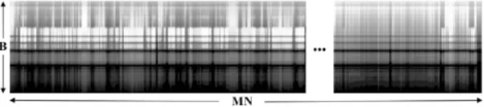
(12)Given the computational efficiency and implementation simplicity, we reshape the 3D HSI cube by concatenating all its vertical spectral slices into a B×MN matrix [15]. The column denotes the spectral reflectance of each pixel, and the row represents the reshaped image of each band. The reshaped Washington DC Mall data in subsection 3.1 is depicted in Fig. 1.
To this end, we arrive at the final cost function with the constraint of the spectral sparsity imposed on the SSAUV model, that is 2 2 2 1 1 1 ( ( ) 2 ˆ ) ( 1 min u f WR u u u B x y u ∇ − + ∇ + − τ τ (13)
FIG. 1. The reshaped Washington DC Mall data.
Here in, W is the weighting matrix, which contains M×N elements. Formula (13) involves two unsmooth and inseparable l1-norm terms. It is difficult to minimize directly. In the next
subsection, we apply the standard split Bregman algorithm [29] to minimize (13) for its efficiency and fast convergence to solve the l1-regularized optimization problem.
2.4. Optimization Procedure
Following Ref. [29], (13) is transformed to the following constrained problem by introducing two auxiliary variables dx and dy, 2 2 2 1 1 1 ( ) 2 ˆ 1 min d WR d u u B x y u + + − τ τ (14) st. dx=∇x(u− f) dy=∇yu
Sequentially, (14) is further converted into an unconstrained minimization problem by using a quadratic penalty function:
2 2 2 1 1 1 ( ) 2 ˆ 1 min , , dy B dx WRdy u u x d u + + − τ τ 2 2 2 2 2 ) ( 2 dx−∇x u−f −bx + dy−∇yu−by +α β (15)
where α and β are the penalization parameters, and bx
and by are the introduced Bregman variables to accelerate
the iteration. The above optimization problem can be decoupled into three subproblems (16), (18) and (20), together with Bregman updates (21).
The u-related subproblem is
2 2 2 2 2 ( ) 2 ˆ 2 min k k x k x u u−u + d −∇ u−f −b α τ 2 2 2 k y y k y u b d −∇ − +β (16)
which is a least-square problem. Nulling the first derivative of (16) yields the following formula
(
)
k k x k x T x k y T y x T x β τ2u 1 α (d f b ) α∇∇ + ∇∇ + + = ∇ +∇ − +β∇Ty(dky−bky)+τ2uˆk (17)which is strictly diagonal and can be solved using the Gauss-Seidel algorithm.
The dx-related subproblem is
2 2 1 1 2 ( ) 1 min k x k x x x dx B d + d −∇ u − f −b + α (18) whose solution is ) 1 , ) ( ( shrink 1 1 α B b f u dkx+ = ∇x k+ − + kk (19)
where in shrink(x, s)=sgn(x) ․ max(-s, 0).
Similarly, the solution to the dy-related subproblem is
(
)
⎟⎟⎠⎞ ⎜⎜⎝ ⎛ ∇ + − + ∇ + ∇ = + + + + max ,0 ) ( 1 1 1 1 1 β τW b u R b u R b u d k y k ky y k y k yj k j y k y (20)Then, we update the Bregman variables as follows:
(
)
⎪⎩ ⎪ ⎨ ⎧ − ∇ + = − − ∇ + = + + + + + + 1 1 1 1 1 1 k y k y k y k y k x k x k x k x d u b b d f u b b (21)Finally, the normalized mean square error (NMSE)
2 2 1 2 2 1 / + + − k k k u u
u is applied as the stopping criterion.
III. RESULTS AND DISCUSSION
To validate the destriping performance, we performed simulations and actual experiments, and compared our method with the combined wavelet-Fourier filter (wavelet-FFT) [5], the variational stationary noise remover method (VSNR) [30], the SSAHTV method [14], and the UV method [10]. For fair comparison, parameters in these algorithms were kept equal for each band. They were tuned until the best performance was obtained.
In all cases, the gray values of HSIs were normalized between [0, 1]. We refer to peak signal-to-noise ratio (PSNR) and structural similarity (SSIM) [31] to quantitatively assess the improvement. The mean indices of all the bands are denoted as MPSNR and MSSIM. Generally, larger index values indicate better restoration results.
3.1. Simulation Results
In this subsection, the Washington DC Mall data, acquired by Hyperspectral Digital Imagery Collection Experiment (HYDICE), was utilized to test the effectiveness of the proposed method. This HSI contained 307 × 307 pixels and 191 spectral bands.
Under the assumption that the raw data was noise-free, the striped images were obtained by adding the same zero-mean Gaussian noise n∈R1×307, with the standard deviation (STD)
(a) (b) (c)
(d) (e) (f)
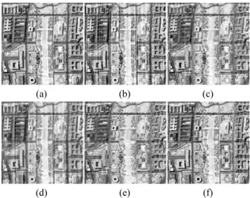
FIG. 2. Destriped results of band 58 in Scenario 1. (a) Original image. (b) Noisy image. (c)Wavelet-FFT. (d) SSAHTV. (e) Proposed model without SR term. (f) Proposed model.
(a) (b) (c)
(d) (e) (f)
FIG. 3. Destriped results of band 156 in Scenario 1. (a) Original image. (b) Noisy image. (c) Wavelet-FFT. (d) SSAHTV. (e) Proposed model without SR term. (f) Proposed model.
(a) (b) (c)
(d) (e) (f)
FIG. 4. Destriped results of band 58 in Scenario 2. (a) Original image. (b) Noisy image. (c) Wavelet-FFT. (d) SSAHTV. (e) Proposed model without SR term. (f) Proposed model.
(a) (b) (c)
(d) (e) (f)
FIG. 5. Destriped results of band 156 in Scenario 2. (a) Original image. (b) Noisy image. (c) Wavelet-FFT. (d) SSAHTV. (e) Proposed model without SR term. (f) Proposed model.
σ , to all the rows at each band. The addition of the stripes was simulated in two different scenarios: (1) For different bands, the magnitudes of stripes were equal, i.e., the STD σ was 0.12 for all the bands. (2) For different bands, the magnitudes of the stripes were different, i.e., the STD σ increased from 0.10 to 0.16 uniformly.
Bands 58 and 156 are selected as typical bands. The results for Scenario 1 are shown in Figs. 2 and 3, and Scenario 2 in Figs. 4 and 5. It is obvious that the proposed method achieves the best destriping results, where the stripes are altogether removed and the structural details are well preserved. In comparison, the band-wise wavelet-FFT method can remove most of the stripes and improve the visual quality of the images, but a few residual stripes still remain as
indicated by the ellipse marks. Even worse, the image contrast is unexpectedly decreased. The results via the SSAHTV model are over-smoothed and exhibit severe loss of details. Although this model has taken into account the differences of the spectral and spatial information, it fails to exploit the directional property of the stripes. Essentially, it is an isotropic model, which accounts for the residual stripes.
The effect of sparse representation (SR) was also investigated. The SR term was removed and the stripes were suppressed in the SSAUV model. The results in Figs. 2(e)-5(e) show that some vertical structures, i.e., the road in the ellipse marks, are degraded together with the stripes, which implies that spectral distortion may be induced. This is primarily because the SSAUV model only emphasizes the
(a) (b) (c) (d)
FIG. 6. Spectrum difference between the noise-free and the destriped image at pixel (100,200) of Scenario 2. (a) Wavelet-FFT. (b) SSAHTV. (c) Without SR. (d) Proposed.
(a) (b) (c) (d)
FIG. 7. Spectrum difference between the noise-free and the destriped image at pixel (300,300) of Scenario 2. (a) Wavelet-FFT. (b) SSAHTV. (c) Without SR. (d) Proposed.
(a) (b)
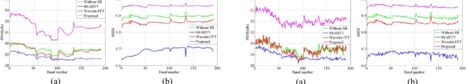
FIG. 8. Band-wise PSNR and SSIM values in Scenario 1. (a) PSNR. (b) SSIM.
TABLE 1. Quantitative evaluation of the simulated experiments before and after destriping
Scenario Index Wavelet-FFT SSAHTV Without SR Proposed
1 M-MPSNR 29.32(0.03) 28.86(0.03) 29.51(0.04) 32.07(0.03)
M-MSSIM 0.8562(0.0005) 0.6929(0.0013) 0.8952(0.0005) 0.9335(0.0005)
2 M-MPSNR 29.47(0.03) 28.85(0.04) 29.54(0.04) 32.11(0.03)
M-MSSIM 0.8563(0.0005) 0.6708(0.0014) 0.8927(0.0006) 0.9552(0.0006)
(a) (b)
FIG. 9. Band-wise PSNR and SSIM values in Scenario 2. (a) PSNR. (b) SSIM.
smoothness perpendicular to the stripes, and the spectral correlation is ignored. For Scenario 2, Figs. 6 and 7 plot the spectrum differences at pixels (100, 200) and (300, 300) of each band, respectively. It is apparent that the proposed method inhibits spectral distortion, benefiting from the sparsity constraint.
Band-wise PSNR and SSIM values of the two scenarios are presented in Figs. 8 and 9. The proposed method
achieves a consistent improvement of over 2 dB in terms of PSNR, illustrating that our method is rather noise insensitive. In addition, the simulations were repeated 10 times using different random noise patterns. The arithmetic mean of MPSNR and MSSIM with their uncertainties, denoted by M-MPSNR and M-MSSIM, is condensed in Table 1. The numbers in parentheses correspond to Type A standard uncertainty. Consistent with the visual performance,
(a) (b) (c)
(d) (e) (f)
FIG. 10. Destriped results of band 96 in EO-1 data. (a) Noisy image. (b) Wavelet-FFT. (c) SSAHTV. (d) VSNR. (e) UV. (f) Proposed.
(a) (b) (c)
(d) (e) (f)
FIG. 11. Destriped results of band 173 in EO-1 data. (a) Noisy image. (b) Wavelet-FFT. (c) SSAHTV. (d) VSNR. (e) UV. (f) Proposed.
the proposed method outperforms other methods in point of PSNR and SSIM values. The simulations have demon-strated the compelling performance of our method in preserving details and suppressing stripes with less spectral distortion, regardless of stripe intensities.
3.2. Actual Results 3.2.1. EO-1 Results
The Earth Observing-1 (EO-1) Hyperion data was acquired by the Hyperion sensor over Hualien County, Taiwan on May 4th, 2005. The original data, with random noise and stripes, was composed of 242 bands in spectrum range of 0.4 to 2.5 mm. Each band contained 256×6974 pixels. After removing some bands with little information, the final test data was cropped to the size of 256×256×149. The band indexes of the test data were 8~57, 77~115, 117~120, 131~133, 135, 138, 140~162, 164, 171~176, 179~180, 182, 184, 195~209, and 222~223, respectively.
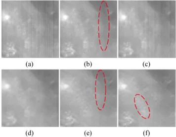
The results of band 96 with tiny stripes are shown in Fig. 10. As the band-wise wavelet-FFT and VSNR methods neglect the spectrally varying intensities of the stripes, the global parameters appear so large for this band that the destriped images are excessively smoothed. Hence, heavy artifacts are introduced. For the SSAHTV method, these slight stripes are removed, without causing noticeable artifacts. The destriped image in Fig. 10(e) seems plausible. However, the UV method focuses too much on the destriping, which leads to loss of useful information.
The results of band 173 with severe stripes are shown in Fig. 11. For the wavelet-FFT method, although most of the stripes are alleviated and visually pleasant results are achieved, some residual stripes persist in the ellipse area marked in Fig. 11(b). For the results via the SSAHTV model, quite a part of stripes can be observed. Even worse, the images appear over-smoothed and suffer from significant
loss of details. Similar results are achieved by the VSNR method. According to the destriping result of UV, this method is less robust than the proposed method, because we can still see stripe artifacts in the ellipse area in Fig. 11(e).
Evidently, our approach provides the best destriping results. The stripes in smooth regions are fully erased, while the detail information is well preserved, which is attributed to the adaptive mechanism in the spatial domain. Furthermore, the spectrally varying intensities of the stripes are sufficiently considered: On one hand, small denoising strengths are enforced to band 96, thus the maximum data genuineness is preserved in Fig. 10(f). On the other hand, large denoising strengths are enforced to band 173, thus the stripes are effectively removed in Fig. 11(f). Besides, benefiting from the sparse representation term, the spectral correlation is exploited and the contrast of the destriped image is not decreased.
Figs. 12 and 13 display the mean cross-track profiles of bands 96 and 173 before and after destriping, respectively. Owing to the existence of the stripes, the curves in Figs. 12(a) and 13(a) exhibit rapid fluctuations. It can be seen that the curves of our results are quite smooth and follow the similar trend as the raw data. For the wavelet-FFT method, the curves appear over smoothed, indicating that the textures are unexpectedly degraded. Even though the fluctuations in Figs. 12(c), 12(d), 13(c), and 13(d) are somewhat suppressed, a few burrs, indicating residual stripes, still remain. For the UV method, the trend of the cross-track profile in Fig. 12(e) differs a lot from Fig. 12(a), which indicates that brightness distortion is introduced in the destriping process.
3.2.2. Urban Results
The Urban scene in Texas was collected by the HYDICE sensor, which could be downloaded online at http://www. tec.army.mil/hypercube. This HSI was ravaged by random
(a) (b) (c)
(d) (e) (f)
FIG. 12. Mean cross-track profiles for the images shown in Fig.10.
(a) (b) (c)
(d) (e) (f)
FIG. 13. Mean cross-track profiles for the images shown in Fig.11.
(a) (b) (c)
(d) (e) (f)
FIG. 14. Destriped results of band 109 in Urban data. (a) Noisy image. (b) Wavelet-FFT. (c) SSAHTV. (d) VSNR. (e) UV. (f) Proposed.
(a) (b) (c)
(d) (e) (f)
FIG. 15. Destriped results of band 204 in Urban data. (a) Noisy image. (b) Wavelet-FFT. (c) SSAHTV. (d) VSNR. (e) UV. (f) Proposed.
noise and stripes simultaneously, and consisted of 307×307 pixels and 210 bands ranging from 0.4 to 2.4 mm. Bands 104-108, 139-151, and 207-210 were abandoned for high degree of noise and little useful information. The remaining test data was 307×307×188 in size.
The destriping results of bands 109 and 204 are presented in Figs. 14 and 15, respectively. Subjectively, the proposed model is superior to the other four contrasting methods. In the band-wise wavelet-FFT method, the damping factor depends on the whole data cube and stays constant for each band. Consequently, for the bands with slight stripes, the constant damping factor is too large to preserve details, as shown in Fig. 15(b). The SSAHTV method is capable of eliminating the slight stripes, as shown in Fig. 15(c), whereas a few severe stripes in Fig. 14(c) still exist since the directional characteristic of stripes is not taken into consideration. Besides, random noise is suppressed to some extent. For the VSNR method and the UV method, the residual stripes are still significant in Figs. 15(d) and 15(e), respectively.
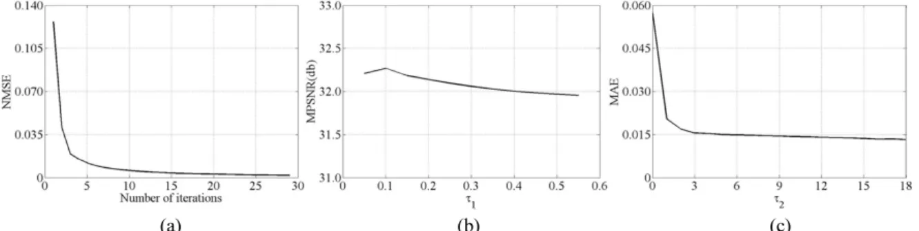
3.3. Convergence Speed and Parameter Selection To measure the convergence speed of the proposed method, Fig. 16(a) plots NMSE as a function of iteration numbers on the simulated experiment Scenario 2. The NMSE curve decreases significantly in the first five iterations due to the efficiency of the split Bregman method. Since the evolution curve converges after about 17 iterations, the maximum number of iterations kmax was empirically set to 20 throughout
the experiments in this paper.
The selection of regulation parameters τ1 and τ2 plays a critical role in the denoising process. To confirm the robustness of the proposed method, we plot the curve of MPSNR versus τ1 on Scenario 2 in Fig. 16(b), and the mean absolute error (MAE) of the spectrum difference at pixel (100,200) versus τ2 in Fig. 16(c), respectively. In Fig. 16(b), MPSNR
(a) (b) (c)
FIG. 16. (a) Curve of NMSE versus iteration number. (b) Curve of MPSNR versus τ1. (c) Curve of MAE of spectrum difference at pixel (100, 200) versus τ2.
values change little with τ1 in the interval [0.05, 0.4]. In addition, as the stripe intensities are different at each band in Scenario 2, it further confirms that our method is robust to the variation of stripe intensities. The robustness is attributed to the adaptive mechanism in the spectral and spatial domain. In this paper, τ1 was fixed to 0.2.
As seen in Fig. 16(c), the MAE curve decreases gradually with the increase of τ2 and keeps almost invariable when
τ2 exceeds 3. That is, the variation of τ2 has little effect
on MAE values, which confirms the robustness over a wide range. Empirically, τ2 was set over 3. Moreover, when
τ2 is equal to 0, the sparsity term is abandoned, and the
proposed model degenerates to the SSAUV model. In this case, the MAE values are about 0.04 higher than that of the proposed method, which further validates the effectiveness of the sparsity regulation. Less spectral distortion is ascribed to that sparse representation can preserve the spectral correlation via dictionary learning in the spectral domain.
To test the parameter η on the proposed model, PSNR values are tested on the simulation experiment when η is selected to be 5, 10, 15, 20, and 25, respectively. PSNR values change little when η varies from 5 to 25, which indicates that the proposed method is robust with the parameter η . Thus, η is fixed to 15 throughout this paper.
Selection principles of the parameters in split Bregman and sparse representation methods are not particularly discussed, as they are beyond the scope of this paper.
IV. CONCLUSION
In this paper, we present a variational method to destripe HSIs. We take the stripe noise properties of unidirection, spectral correction, and variation of stripe intensities in different bands and regions into full consideration. Instead of manual selection band by band, regulation parameters adapt to the spectrally varying intensities of stripes and the spatially varying texture information. Moreover, spectral correlation is exploited via the sparse representation constraint to prevent spectral distortion. Then, the split Bregman method is employed to optimize the minimization problem. Experiment results demonstrate that the proposed method
can remove the stripes in different bands and different regions efficiently, without distortion in the spectral domain and loss of structural details. In addition, the proposed method is robust to parameter selection and stripe intensities.
The proposed method may be computationally complex, as any iterative algorithm. Future extension of this work may include speeding up the method with parallel techniques, such as graphic processing units (GPUs). Destriping, as well as deblurring, dehazing, and super resolution is a typical inverse problem. It may be interesting to tackle these issues simultaneously in one framework.
ACKNOWLEDGMENT
This work is funded by the National Natural Science Foundation of China (NSFC) (61308099).
REFERENCES
1. J. Bioucas-Dias, A. Plaza, G. Camps-Valls, P. Scheunders, N. Nasrabadi, and J. Chanussot, “Hyperspectral remote sensing data analysis and future challenges,” IEEE Geosci. Remote Sens. Mag. 1, 6-36 (2013).
2. K. Mikelsons, M. Wang, L. Jiang, and M. Bouali, “Destriping algorithm for improved satellite-derived ocean color product
imagery,” Opt. Express 22, 28058-28070 (2014).
3. J. Chen, Y. Shao, H. Guo, W. Wang, and B. Zhu, “Destriping CMODIS data by power filtering,” IEEE Trans. Geosci.
Rem. Sens. 41, 2119-2124 (2003).
4. R. Pande-Chhetri and A. Abd-Elrahman, “De-striping hyper-spectral imagery using wavelet transform and adaptive frequency
domain filtering,” ISPRS J. Photogramm. Remote Sens. 66,
620-636 (2011).
5. B. Münch, P. Trtik, F. Marone, and M. Stampanoni, “Stripe and ring artifact removal with combined wavelet-Fourier filtering,”
Opt. Express 17, 8567-8591 (2009).
6. J. Torres and S. O. Infante, “Wavelet analysis for the elimination of striping noise in satellite images,” Opt. Eng. 40, 1309-1314 (2001).
7. J. Chen, H. Lin, Y. Shao, and L. Yang, “Oblique striping removal in remote sensing imagery based on wavelet transform,”
Int. J. Remote Sens. 27, 1717-1723 (2006).
8. B. K. Horn and R. J. Woodham, “Destriping Landsat MSS images by histogram modification,” Comput. Graph. Image
Process. 10, 69-83 (1979).
9. M. Weinreb, R. Xie, J. Lienesch, and D. Crosby, “Destriping GOES images by matching empirical distribution functions,” Remote Sens. Environ. 29, 185-195 (1989).
10. M. Bouali and S. Ladjal, “Toward optimal destriping of MODIS data using a unidirectional variational model,” IEEE Trans. Geosci. Rem. Sens. 49, 2924-2935 (2011).
11. Y. Chang, H. Fang, L. Yan, and H. Liu, “Robust destriping method with unidirectional total variation and framelet regularization,” Opt. Express 21, 23307-23323 (2013). 12. J. I. Sperl, D. Bequé, G. P. Kudielka, K. Mahdi, P. M.
Edic, and C. Cozzini, “A Fourier-domain algorithm for total-variation regularized phase retrieval in differential X-ray phase contrast imaging,” Opt. Express 22, 450-462 (2014). 13. G. Gong, H. Zhang, and M. Yao, “Construction model for
total variation regularization parameter,” Opt. Express 22,
10500-10508 (2014).
14. Q. Yuan, L. Zhang, and H. Shen, “Hyperspectral image denoising employing a spectral-spatial adaptive total variation model,”
IEEE Trans. Geosci. Rem. Sens. 50, 3660-3677 (2012).
15. Y.-Q. Zhao and J. Yang, “Hyperspectral image denoising via sparse representation and low-rank constraint,” IEEE Trans.
Geosci. Rem. Sens. 53, 296-308 (2015).
16. Y. Chang, L. Yan, H. Fang, and H. Liu, “Simultaneous destriping and denoising for remote sensing images with unidirectional total variation and sparse representation,” IEEE Trans. Geosci. Rem. Sens. 11, 1051-1055 (2014).
17. N. Cao, A. Nehorai, and M. Jacobs, “Image reconstruction for diffuse optical tomography using sparsity regularization
and expectation-maximization algorithm,” Opt. Express 15,
13695-13708 (2007).
18. E. Y. Sidky, M. A. Anastasio, and X. Pan, “Image recon-struction exploiting object sparsity in boundary-enhanced X-ray phase-contrast tomography,” Opt. Express 18, 10404- 10422 (2010).
19. M. Elad and M. Aharon, “Image denoising via sparse and redundant representations over learned dictionaries,” IEEE Trans. Image Process. 15, 3736-3745 (2006).
20. A. Kostenko, K. J. Batenburg, H. Suhonen, S. E. Offerman, and L. J. van Vliet, “Phase retrieval in in-line x-ray phase contrast imaging based on total variation minimization,” Opt. Express 21, 710-723 (2013).
21. M. Freiberger, C. Clason, and H. Scharfetter, “Total variation regularization for nonlinear fluorescence tomography with an augmented lagrangian splitting approach,” Appl. Opt. 49, 3741-3747 (2010).
22. A. Kostenko, K. J. Batenburg, A. King, S. E. Offerman, and L. J. van Vliet, “Total variation minimization approach in in-line x-ray phase-contrast tomography,” Opt. Express 21, 12185-12196 (2013).
23. Y. Y. Schechner and Y. Averbuch, “Regularized image recovery in scattering media,” IEEE Trans. Pattern Anal. Mach. Intell. 29, 1655-1660 (2007).
24. X. Bresson and T. F. Chan, “Fast dual minimization of the vectorial total variation norm and applications to color image
processing,” Inverse Probl. Imag. 2, 455-484 (2008).
25. E. Vera, P. Meza, and S. Torres, “Total variation approach for adaptive nonuniformity correction in focal-plane arrays,” Opt. Lett. 36, 172-174 (2011).
26. J. Axelsson, J. Svensson, and S. Andersson-Engels, “Spatially varying regularization based on spectrally resolved fluorescence emission in fluorescence molecular tomography,” Opt. Express 15, 13574-13584 (2007).
27. Q. Chen, P. Montesinos, Q. S. Sun, P. A. Heng, and D. S. Xia, “Adaptive total variation denoising based on difference curvature,” Image Vis. Comput. 28, 298-306 (2010). 28. S. Mallat and Z. Zhang, “Matching pursuits with time-
frequency dictionaries,” IEEE Trans. Signal Process. 41, 3397-3415 (1993).
29. T. Goldstein and S. Osher, “The split Bregman method for
L1-regularized problems,” SIAM J. Imag. Sci. 2, 323-343
(2009).
30. J. Fehrenbach, P. Weiss, and C. Lorenzo, “Variational algorithms to remove stationary noise: Applications to microscopy imaging,” IEEE Trans. Image Process. 21, 4420-4430 (2012). 31. Z. Wang, A. C. Bovik, H. R. Sheikh, and E. P. Simoncelli,
“Image quality assessment: From error visibility to structural