Vol.22, No.4, (2020), pp.31~39 https://doi.org/10.9714/psac.2020.22.4.031
```
1. INTRODUCTION
The power transmission cables are definitely the most advanced ones among possible applications of high temperature superconductors (HTS) for electro-energetics. In the most comprehensive review [1] thirty HTS power cables are listed that are developed, tested, projected or installed in grids. HTS cable applications for grids are discussed in [2]. Some projects are already considered as the commercial ones [3].
Up to now most cables produced, successfully tested and installed to electrical grids worldwide are made of the First Generation (1G) HTS wires [1]. Power cables made of the Second Generation HTS wires (2G or Coated Conductors) are in active development and testing, but still not widely introduced yet. Most probably due to more expensive 2G wires in comparison with 1G wires.
The basic principles of 1G HTS power cables development have been published in many works since 90-ties, for example [4-10]. The most attention has been paid to providing of uniform current distribution between layers that is important for an achievement of full use of superconducting properties in multilayer HTS cables [9].
We have to note, that the problem of uniform current distribution between layers is important just for AC cables. In DC cables current distribution is determined by joint resistances with terminations and is not crucial. On the other hand, AC cables, that are more important for common
power grids, current distribution between layers is determined by full impedances of layers, which must be the same for each layer. This should be achieved by providing the certain twist pitch and twist direction of layers [9].
For future applications 2G HTS cables are more promising than 1G HTS cables due to their higher current density, lower AC losses and less anticipated cost with mass-production developed. Thinner 2G HTS tapes are much more flexible than 1G tapes, allowing smaller bending diameter. Thus, the smaller cables diameter could be implemented with making 2G HTS power cables more compact and efficient than 1G HTS cables. To keep transport current large enough to provide power necessary, more superconducting layers should be used in compact cables. That makes the problem of uniform current distribution between layer more complicating for 2G AC cables.
In our opinion, some new approaches in modeling, design and production of 2G power cables should be developed and implemented especially for compact HTS cables.
In Russian Scientific R&D Cable Institute the research project is underway to reduce as much as possible mass and dimensions of HTS power cables. This is important for such applications as electrical aircrafts, ship propulsion system or other transport applications. Reduction of the diameter makes the allowable cable bending diameter less, that is also important for transport applications with limited space.
Review of the design, production and tests of compact AC HTS
power cables
S. S. Fetisova, V. V. Zubkoa, A. A. Nosova, S. Yu. Zanegina, and V. S. Vysotsky*,a,b
a Russian Scientific R&D Cable Institute, Moscow, Russia
b National Research Nuclear University MEPhI (Moscow Engineering Physics Institute), Moscow, Russia.
(Received 13 November 2020; revised or reviewed 19 December 2020; accepted 20 December 2020)
Abstract
Power cables made of high temperature superconductors (HTS) are considered as most advanced applications of superconductivity for electro-energetics. Several cables made of the First Generation (1G) HTS wires have been produced and installed to electrical grids worldwide. Power cables made of the Second Generation HTS wires (2G or Coated Conductors) are in active development. Most basic principles of HTS power cables development have been published in many works since 90-ties. In this Review we would like to present our new developments mostly directed to 2G HTS compact power cables. We are presenting the methods to optimize a design of 2G AC compact power cable providing uniform current distribution among cable layers and the production technology approaches to implement such a design. AC losses measurements in such cables and other test methods are described. Some problems of the development 2G HTS power cables with small diameters are discussed. We presented as examples designs, developments and test results of two major coaxial cables designs: single-phase (cable core and a shield) and three-phase (triaxial: with three coaxial phases).
Keywords: HTS cables design, HTS Modeling, HTS cables, AC losses
In this Review we are presenting our recent developments in design, modeling, production and testing that intended for the development of 2G HTS compact power cables. First, we are describing the advanced approaches on design optimization of 2G AC power cable, particularly by use of Finite Element Methods (FEM) that permitted precise calculations to provide uniform current distribution between layers. These methods are important in designing of compact cables with a small diameter when thickness of a superconducting layer is not too small in comparison with a diameter of a cable. The production technology to implement a design with precise twisting parameters necessary to keep uniform current distribution between layers is also considered. AC losses measurements in 2G cables and other test methods are described.
Our approaches are illustrated and validated with use of examples of compact 2G HTS cables prototypes with small diameters developed and tested experimentally. We are presenting results for two coaxial cables designs: single-phase (cable core and a shield) and three-phase (triaxial: with three coaxial phases).
2. METHODS TO OPTIMIZE A DESIGN OF THE 2G AC COAXIAL CABLES
The methods to calculate the optimal design in 1G HTS AC cables were discussed earlier [3-7]. The use of 2G HTS tapes and especially for cables with small diameter demands more precise calculations. Two approach can be used for coaxial HTS cables design optimization.
2.1. Electric Circuit Models
Our first approach is using the electric circuit models of the cable with current or voltage sources feeding the circuit where a multi-layer core and HTS shield of the cable can be modelled as electric parallel of different branches, one for each layer of superconducting tapes (taking into account that layers in a cable are electrically insulated).
For example, the Kirchhoff equations for electric circuit model with a current source are presented below:
1 1, 1, 1 1, 1 ,1 , 1 , 1,1 1, 1 1, 1 ,1 ,1 ,1 , , 1 , m m N add add m m m m m N m add add m m m m m N m addSc addSc N N m N m N N addSc n M M M M dI dt R I M M M M dI dt R I M M M M dI dt R I M M M M dI dt R , 0 addSc n I (1)
m i total add i t I I t I 1 ) ( ) ( (2) ,I
N(
t
)
I
addScn
0
(3)where t – time, m is number of the layers in core, n is number of the layers in shield, N=m+n, ΔIi – is a current
change in the layer, Mk and Mk,j – are the self-inductance of
the layer and the mutual inductance between layers, Itotal(t)
– total current in the cable, Radd, Iadd – the resistance of the
additional branch for the core and the corresponding
current, RaddSc,i, IaddSc,i – the resistance of the additional
branches for each layer in the shield and the corresponding currents.
This model is implemented by adding branch with a very large resistance in parallel to the all layers of the core (like in [10]) and by adding branches with very small resistances in parallel to each layers of the shield.
The Mk - self-inductances of the layer and Mk,i - the
mutual inductances between k and i layers are calculated by the expressions [11]: 2 0 0 2 1 ln 2 s k k k k r M r r L
(4)μ0 - is the magnetic permeability of vacuum, rk is the inner
radius of the k layer, rs is the distance between the cable
center and the outmost surface, Lk is the twist pitch of the k
layer. 2 0 , 0 1 1 ln 2 s k i i k i k i k r M a a r r L L
(5)
(5)
where ai and ak are constants (+1 or -1), considering the
relative winding direction (clockwise or anti-clockwise). The problem of solving any system of equations can be formulated as the task of minimizing the objective function. In our case, the problem of determining the uniform distribution of currents between the core layers and shield layers of the cable can be formulated as:
1 1 1 1 1 1 min m m N N k i k i k i k k m i k F Х f Х I X I X I X I X
(6) (6)where Ik – the maximum values of currents in the layers
obtained from the solution of equations (1-3),
1, , , , , , , ,1 1 2 2 2 N N, N
Х r L a r L a r L a – vector of the optimized
variables, rk – inner radius of layers, ak is winding direction
of HTS tapes in a layer, Lk is the pitch length of the k layer.
The constraints on the rk, ak, Lk values is the conservation of
the superconductivity state in HTS tapes.
2.2. Finite Element Methods of Optimization of Coaxial HTS Cables
The second approach is using 3D models of the finite element method (FEM).
Two FEM models have been developed, using the ANSYS Emag [12] software for solving the transient electromagnetic problem for complex study of the 2G HTS cable.
The detailed FEM model offers the possibility to modelling any topology of a HTS cable. So, the 3D model permits taking into account the spiral structure of a cable core and shielding layers to obtain current and magnetic field distribution inside a cable. However, the problem is that the task is too complicated and takes a lot of computing time to perform calculations. Thus, the FEM model could be only used to test the optimized variables of the cable.
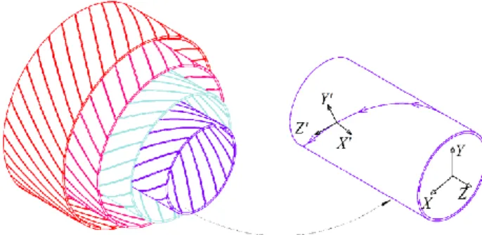
In Fig. 1 the mesh elements in detailed 3D model of the layers of HTS tapes are shown on the end part of the compact
Fig. 1. The mesh elements in detailed 3D FEM model of the layers of HTS tapes on the end part of the cable (4-layers in the core and 2-layers in the shield).
compact 2G HTS cable. The cable consists of four layers in the core and two layers in the HTS shield.
For faster calculations the simpler 3D FEM model has been developed to simulate spirally wound HTS layers as thin cylinders with anisotropy of the electrical conductivity. In this model, a cable core and a shielding layer of the cable are modeled by a system of thin concentric layers (cylinders) where all superconducting layers are isolated from each other (Fig. 2).
In superconducting thin cylinders, the winding direction and twist pitch of the HTS tapes are modeled as the anisotropy of the electrical conductivity.
The electrical conductivity of the anisotropic thin conductor is a tensor of order two, where all off-diagonal elements are zero. In coordinates x,’ y,’ z' a tensor has the form: ' ' ' 0 0 0 0 0 0 z y x
, (7)where σx′ = σy′ ≠ σz′ – electrical conductivity in the
coordinates indicated, z' is a coordinate parallel to winding direction of the superconducting tape in the layer.
In this case, the problem of obtaining a uniform current distribution in the cable core and in the shield can be formulated as the task of minimizing the objective function (6). In this function the maximum values of the currents in the layers are calculated by this model on the basis of the finite element method, and the optimized variables are the direction of electric conductivity σz′ for each cylinder.
Fig. 2. Modeling of HTS layers by thin cylinders.
2.3. Optimization and Design of the Triaxial HTS Cable Triaxial High Temperature Superconducting (HTS) AC power cable, that incorporates three HTS phases wound around a single core within a single cable is the optimal solution for low and medium voltages. This design permits to save expensive HTS wires and to increase the power density transmitted. The advantages of triaxial cables were proved by large scale Bixby and AmpaCity projects [13, 14]. These triaxial cables used one HTS layer made of Bi-2223 tapes per each phase. Similarly, one HTS layer made of ReBCO HTS wires have been developed and tested in Russian Scientific R&D Cable Institute [15]. This cable has been successfully tested and demonstrated about 20 times less AC losses than the power cable with the same parameters made of 1G HTS wires [15].
It is difficult to increase the transmission capacity of a triaxial cable by increasing its operating voltage and, therefore, an insulation thickness between phases. The other way is to increase the operation current by using a multilayer structure in each phase of the cable. This task demands a complicated optimization analysis to provide proper current distribution between phases and tape layers in each phase.
As well as for coaxial cable, to optimize the distribution of currents between layers in the phases of the triaxial cable, numerical models based on an equivalent electrical circuit and a three-dimensional model that uses the finite element method have been developed.
For optimization of the current carrying element of triaxial three phase HTS cable to calculate currents and voltages in phases based on equivalent electrical circuit we used the standard mathematic equations:
, , 1 , , 1 ( , ) ( ) ( ) ( , ) p p N k i k k k k k i i N k i k k i i dI U t z R I I t M z dt dU I t z C z dt
(8) (8)where N – number of layers; Mk и Mki - self-inductances of
layers and mutual-inductances between layers; Ik, Uk and dIk/dt – current, voltage and velocity of a current change in
each layer correspondingly; R(Ik) – resistance of a layer
dependent on a current; Сki- electrical capacitance between
layers.
The self-inductances of layers and mutual inductances between layers per unit length, were found by calculating the expressions (4-5).
The capacitances between layers of the cable were found by calculating the expression:
i k k ir
r
ln
2
C
r 0 ,
(9) (9) where ri is the radius of the inner phase, rj is the radius ofthe outer phase, ε0 is the permittivity of the free space, and εr is the relative permittivity of the dielectric material.
The maximum current values in the layers of each phase should be equal to each other, for example, for phase A:
, , , 1 1
,
N A A A i A i A i iI
I
I
I
I
N
(10) (10)In addition, in order to the currents and voltages in the phases (A, B, C) of the cable to be balanced, their values must satisfy the following conditions:
2 2 , , , , exp( 2 / 3) В А С A B A C A I I I I V V V V j (11)
where j is the imaginary unit.
Two FEM models have been also developed using the ANSYS Emag software for complex study of the triaxial 2G HTS cable.
Again, for faster calculations the 3D FEM model with simple geometrical configuration has been developed, in which layers in the phases of the cable are modeled by a system of thin concentric layers (cylinders) where all the layers are isolated from each other. In superconducting thin cylinders, the optimized variables (the winding direction and twist pitch of the HTS tapes) are modeled by the anisotropy of the electrical conductivity of each cylinder. The detailed 3D FEM model was also used to verify the result of the optimization. This model offers the possibility to model any topology of the HTS cable. The model allows considering the spiral structure of the layers to obtain current and detailed magnetic field distribution inside the cable.
In Fig. 3, the mesh elements in detailed 3D model of the HTS tape layers is shown on the end part of the triaxial cable. The cable contains two layers in each phase.
2.4. Influence of Manufacturing Imprecision on Current Redistribution between Layers
As it was mentioned above, the reduction of the cable diameter will demand to increase of the number of superconducting layers both in a cable core and a cable shield to keep the transferring power in a cable. In [16] a sufficient inhomogeneity of current distribution has been
Fig. 3. The mesh elements in detailed 3D FEM model of the layers of HTS tapes on the end part of the triaxial cable. Letters A, B, C indicate the phases of the cable.
Fig. 4. Cost of manufacturing imprecision in diameters. Relative currents of layers are shown as ratio of current in the layer to the total current [17].
demonstrated between layers in the compact cable (inner diameter 11.3 mm, outer diameter 19.6 mm) because of a small manufacturing inaccuracy. Securing uniform current distribution between the core layers as well as between the shield layers in a multilayer cable is the sophisticated task for cables with small diameters. High precision methods both for the optimization and manufacturing of compact cables are necessary [16]. The numerical optimization methods described above permit analysis of the influence of an insufficient accuracy with reference to compact cables.
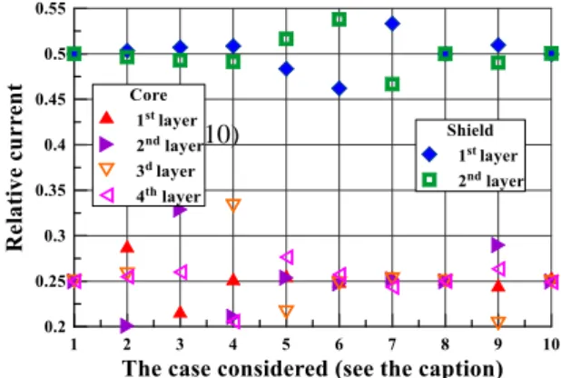
The analysis of sensitivity of current distribution to manufacturing inaccuracy for the cable with inner diameter ~10 mm has been performed in [17]. We determined how changes in a layer diameter or in a twist pitch against the optimized values could change the optimized current distribution. In Fig. 4 the calculated relative current changes for 10 cases are shown, when radius of a layer has been slightly changed from optimized value by the thickness of the tape (0.105 mm). In Fig. 5 the calculated relative current changes for 10 cases are shown, when a twist pitch has been changed by 2 mm from optimized twist pitch value.
1- optimized diameter of all layers; 2 -7 - diameter of each layer is increased by the thickness of the tape (2- first layer, 3 – second layer, etc., 6 and 7 - inner and outer layers of the shield correspondingly); 8 - diameters of first and second layers are increased by the thickness of the tape; 9 - diameters of third and fourth layers are increased by the thickness of the tape; 10 - diameters of all layers in the core are increased by the thickness of the tape.
One can see, that manufacturing imprecision in a diameter has much more influence on current distribution than that in a twist pitch. We also have to say that an imprecision in diameter of a shield does not affect the distribution of current in a core. From Fig. 4 and Fig. 5 we can find out in which layer the mistake in a diameter or in a twist pitch has more influence on the final current distribution.
These results demonstrate that besides the fine calculation and optimization methods the special measures must be implemented to provide precise layering during 2G HTS cable manufacturing.
Fig. 5. Cost of manufacturing imprecision in twist pitch. Relative currents of layers are shown as in Figure 4.
2.5. Conclusion to the Section 2
The new methods to optimize the 2G HTS cable design have been developed that are more precise that the previously developed ones [4-10]. Combination of two methods: electric circuit models and calculations with use of FEM permit us to make fine analysis and optimization of HTS cables with small diameters. We also demonstrated how manufacturing imprecision could affect current distribution between layers in a multilayer HTS cable [17]. The validation of these methods will be demonstrated in the next sections.
1-optimized twist pitch in all layers; 2 -7 - twist pitch of one of each layers is increased by 2 mm (2 – first layer, 3 – second layer, etc., 6 and 7 inner and outer layers of the shield correspondingly); 8 - first and second layers twist pitches are increased by 2 mm; 9 - third and fourth layers twist pitches are increased by 2 mm; 10 – twist pitches of all layers of the core only are increased by 2 mm.
3. PRODUCTION AND TESTS METHODS OF HTS CABLES
3.1. Production of Cables Prototypes
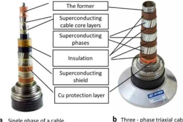
Standard phase of an HTS superconducting cable consists of the following parts (Figure 6 a):
Central former that usually has a tube for cryogen flow and some copper for protection of a cable core in case of a fault with overcurrent;
Several layers of HTS tapes, each of them has to have precise diameter and twist pitch calculated during optimization;
Insulation layer with required thickness;
Superconducting shield that could have several layers as well;
Outer protection copper layer.
In case of a triaxial cable each phase is placed coaxially separated by several insulation layers (Fig. 6 b). Outer shield is not necessary because phases of a triaxial cable are balanced without external magnetic field generation.
Fig. 6. General view of HTS power cables (made of 1G wires). a - single phase of a standard coaxial cable with a shield [16]; b – a triaxial cable with three coaxial phases [13].
Fig. 7. Example of a triaxial HTS cable [10] production process. a – preparation of a former for the inner layer of a triaxial cable (see Figure 6); b - placing of HTS tapes to a cable layer.
As an example, the cable production process for triaxial cable (Fig. 6, b) is shown in Fig. 7 a, b. During the fabrication of a former the inner tube was insulated by crepe cable paper to provide a diameter necessary to support an inner layer of a cable (Fig. 7 a). Then proper number of HTS tapes were placed on a support as it is shown in Fig. 7 b. After the first layer installed it was insulated by few layers of a crepe cable paper.
As we mentioned above it is important to keep a precise diameter and a twist pitch in each layer of the cable with a small diameter. To get the proper current distribution in our multilayer cables during manufacturing, we measured the actual average diameter of each layer wound. Then we recalculated the parameters of the next layer to refine a twist pitch of the following layer. This method permitted us to get the proper current distribution in our compact cables. It is important also to have stiff enough former and insulation that do not change their diameters during cabling.
3.2. HTS Cables Test Methods
The standard test program for model cables in Russian Scientific R&D Cable institute includes (but not exhausted):
DC test to determine critical currents in each layer/phase;
AC test to determine current distribution between layers at AC conditions;
Fig. 8. General view of the facility for testing the cables in Russian Scientific R&D Cable Institute. The test facility includes: 5 m flexible cryostat, DC power supplies up to 4-6.5 kA, Data Acquisition System (DAS) with up 20 000 samples per 50 Hz cycles providing high accuracy digital measurements, amplifiers, flow meters, non-inductive shunts, etc.
The test facility for testing of HTS cable models is shown in Fig. 8. The test methods were earlier described in details [17-22]. Critical currents were determined by measurement of voltage – current characteristics with
1V/cm criteria for the critical current. Current distribution
between layers was determined by the signals from Rogovski coils installed on layers of a cable tested. AC losses were measured by the electrical method when voltage V and current I are measured with high resolution. By the definition, the losses P(t) at the single-phase AC conductor with the current I(t) and voltage V(t) are described as:
(12)
(13) By using of high-resolution data acquisition system
shown in Fig. 8 for V(t) and I(T) measurements, we were able to perform precise digital integration of the products of voltages by currents and to get proper AC loss data. [19].
The results of experimental study of two model cables are presented in the next sections as examples.
4. DEVELOPMENT AND TESTS OF THE COMPACT COAXIAL CABLES PROTOTYPES
In this section we present, as examples, the development and test results of two model cables with small diameters made of 2G HTS wires.
4.1. Single Phase Coaxial Cable with Four Layers in the Cable Core and Two Layers in the Shield
For this cable, we used 2G HTS tapes produced by SuperOx Company [23] with the total thickness of the tapes ~ 0.105 mm. In order to reduce the polygonality of the layers in the core we used the HTS tapes with 3 mm width. Average critical current of these tapes in the self-field at
77.4K is ~80 A. For the shield we used the 2G HTS tapes with 4 mm width. Their average critical current in self-field at 77.4K is ~ 120 A.
4.1.1. Optimization Results
We performed the optimization by use of electric circuit model mentioned above in section I. The results of optimization were compared with calculations by 3D FEM model.
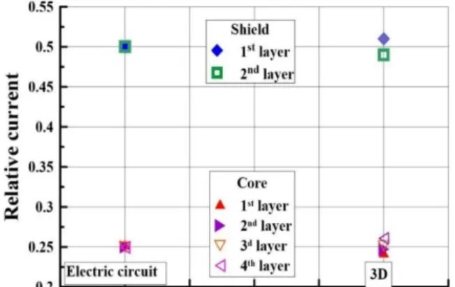
In Fig. 9 the comparison if calculations by 3D FEM method (right) and by electrical circuit method (left) are shown as relative current in a layer, i.e., as a ratio of current in a layer to a total current in a cable. One can see a good coincidence of calculations by two methods that permits us using simplified electrical circuit method for optimization. Then we performed the analysis of sensitivity of current distribution to manufacturing imprecision. We determined how changes in a diameter of a layer or in a twist pitch affects the current distribution (see section 2.4).
The final optimized parameters of the core and the shield for this cable are listed in the Table 1. To provide the minimal AC loss in the cable we must have as small as possible gaps between tapes in cable layers [15]. To achieve this, two tapes were added to second and third layers of the core and one tape was added to outer layer of the shield.
The magnetic field distribution in the cable is shown as an example in Fig.10 when the total current in the cable is 2000A.
Fig. 9. Results of optimization and comparison of calculations by the 3D FEM method and by the electrical circuit method.
TABLE 1
PARAMETERS OF THE CABLE PROTOTYPE. Number of the layer Dmin, mm Twist Pitch, mm Number of tapes Gap between tapes, mm 1 10.32 - 56.2 9 0.15 2 11.03 - 193.6 11 0.12 3 12.03 94.3 11 0.21 4 13.06 40.7 9 0.32 5 18.25 349.4 13 0.36 6 19.06 - 317.4 14 0.22
Fig. 10. Calculated magnetic field distribution at the 2000 A total current in the cable.
4.1.2. Experimental Results
The critical currents (Ic), were determined by the
criterion of 1 μV/cm for each layer at 77.4 K. In the core we got: first layer -729 A; second layer - 891 A; third layer - 895 A; and fourth layer - 735 A or 3250 A in total that is slightly more than expected ~ 3200A. In the shield critical currents were: inner layer -1560 A; outer layer - 1660 or 3220 A in total that is very close to the expected ~ 3240 A. Thus, we can to conclude that in our cable there is no degradation of the critical current due to mechanical stress in the HTS tapes after manufacturing.
The relative currents (ratio of current in layers to total current) obtained from the measurement are shown in Fig. 11. One can see, that as the result of optimization and manufacturing technology used, we were able to achieve practically uniform current distribution among cable layers. Uniformity of currents in the cable core is better than 10% and, in the shield, better than 5%. Slight deviation from uniformity most probably relates to current leads influence. To compare AC losses in this model compact cable with those measured in HTS model cables tested before we performed AC losses measurement by the electrical method described in [22]. In Figure 12 the AC losses in the cable core and the cable shield are shown recalculated per one tape. For comparison, the measured AC losses are shown in
Fig. 11. Measured relative current distribution in layers of the cable core and the shield of the HTS cable versus amplitude of the total current.
Fig. 12. Comparison of AC losses per tape versus relative current in layers of the single-phase compact model cable and AC losses per tape in the shield of compact cables produced and tested in the Russian Cable Institute earlier [16].
the shield of compact 2G HTS cable we produced and tested earlier [16]. AC losses in a core are practically the same as in our first compact cable described in [16], while in the core AC loss are slightly less in this cable. In any cases AC losses in 2G HTS cables are sufficiently less than in 1G HTS cables, for example described in [22].
4.2. Development of the Triaxial Cable with Two Layers per Phase
To manufacture this cable, we used the second generation HTSC tape produced by SuperOx with a total thickness of ~ 0.105 mm and a width of 4 mm. The critical current of these tapes in self-field at a temperature of 77.4 K is ~130-150 A.
4.2.1. Optimization Results
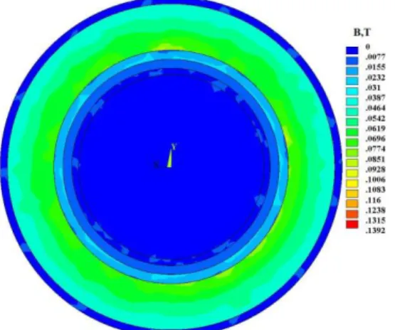
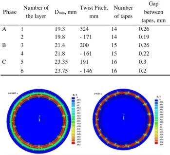
Same as we did before, we performed optimization using the equivalent electrical circuit of the cable, and then the optimization results were compared with the calculations of the 3D FEM model. The central supporting element (former) consisting of copper wires, here is playing the role of the main power element when installing (pulling) the cable into the cryostat, and performs the function of an electric shunt in emergency operating modes of the HTS cable. The former is covered with polyimide tape to insulate it and to level the surface. The final optimized cable parameters are listed in the Table 2. The sign in the twist pitch column indicates the direction of tapes twist. To ensure minimum AC losses, it is necessary to provide the smallest possible gaps between the tapes in the cable layers. As an example, in Fig. 13 the magnetic fields in the cable are shown calculated by the FEM model for two times (0.005 sec and 0.01 sec). One can see that there is no magnetic fee outside the triaxial cable. That is why triaxial cables do not need outer superconducting shield. It means three phase triaxial cables need two times less superconducting wires in comparison with usual three single-phase coaxial cables.
TABLE 2
PARAMETERS OF THE MODEL TRIAXIAL CABLE. Phase Number of
the layer Dmin, mm
Twist Pitch, mm Number of tapes Gap between tapes, mm A 1 19.3 324 14 0.26 2 19.8 - 171 14 0.19 B 3 21.4 200 15 0.26 4 21.8 - 161 15 0.22 C 5 23.35 191 16 0.3 6 23.75 - 146 16 0.2
Fig. 13. The calculated magnetic fields in the cable calculated by the FEM model for two times: left - 0.005 s., right - 0.01 s.
4.2.2. Experimental Results
Critical currents of the cable layers (Ic) were determined
by measuring the voltage-current characteristic for each layer according to the criterion of 1 µV/ cm at a temperature of 77.4 K. The following values of Ic were obtained: the
first layer -1969 A; the second layer - 2070 A, total in phase A - 4039 A; third layer - 2192 A; the fourth layer - 2011 A, total in phase B - 4203 A; the fifth layer -2003 A; the sixth layer – 2016, total in phase C - 4019 A. The experimental values of critical currents in the layers are close to the expected from calculations. It means that during manufacturing of the cable (twisting of the tapes when they are placed to layers) there was not decrease of the critical current in the HTS tapes due to mechanical deformation.
As an example, Fig. 14 shows the measured currents in the phases of this model cable at a frequency of 50 Hz. The maximum currents in the layers of phases practically coincide, however, there is a slight shift between the currents of the layers of each phase (about 5-8 degrees in relation to the optimal values).
Fig. 14. The measured currents in the phases of the triaxial cable at 50 Hz frequency.
Fig. 15. The ratio of the maximum current in the inner layer of each phase to the current in the outer layer depending on the frequency.
The measurements of currents were carried out at different frequencies. Fig. 15 demonstrates the ratio of the current in the inner layer to the current in the outer layer for all phases of the cable versus frequency. One can see that by using our optimization methods and manufacturing technology. We managed to achieve almost uniform current distribution among the layers in phases. Small deviations from uniformity at maximum currents and phase shifts are most likely associated with the influence of current leads.
4.3. Conclusion to the Section IV
In this section we presented the results of design, producing and tests of two types of compact coaxial HTS power cables: single phase cable and triaxial cable. Critical currents, current distribution between layers of cables, AC losses, etc. have been measured. Both cables demonstrated all parameters coincided with calculated and expected. This validated the design and production methods developed.
5. CONCLUSION
In this Review the recent developments in design, modeling, production and testing of 2G HTS AC compact power cables are presented. Two advanced methods to optimize a design of HTS compact power cables by use of Electrical Circuit Model and Finite Element Methods are developed that permitted precise calculations to provide uniform current distribution among layers. The methods could be used especially for the development of compact cables with a small diameter when a thickness of a superconducting layer is not too small in comparison with a diameter of a cable. The production technology to implement a compact cable with a design demanding precise twisting parameters necessary to keep uniform current distribution among layers are also considered. Test facility and test methods are presented as well. The design methods were experimentally verified by development and tests of two 2G HTS compact power model cables. Single phase coaxial cable has fours layers in the core and two layers in the shield. Three phase triaxial cable has two
layers per phase that is the first known triaxial with two layers per phase made of 2G HTS wires.
The experimental results are well coincided with calculations and fully confirmed the adequacy of our optimization and production methods.
ACKNOWLEDGMENT
Part of this work was supported by the Russian Scientific Foundation under Grants 16-19-10563 and 16-19-10563П. Authors would like to express their gratitude to Dr. L.V. Potanina for her help in preparation of this review.
REFERENCES
[1] D. I. Doukas, IEEE Trans. Appl. Supercond., vol. 29, pp. 5401205, 2019.
[2] A. P. Malozemoff, J. Yuan, C. M. Rey, Superconductors in the
power grid. Materials and Applications, edited by C. Rey,
Woodhead Publishing Series in Energy, vol. 65, pp. 133-188. 2015
[3] C. Lee, H. Son, Y. Won, et al., Supercond. Sci. Technol., vol. 33, pp. 044006, 2020.
[4] V. E. Sytnikov, et al., Physica C, vol. 310, pp. 357-363, 1998. [5] P. I. Dolgosheev, V. E. Sytnikov, and G. G. Svalov, Physica C,
vol. 310, pp. 367-373, 1998.
[6] B. Turk, Cryogenics, vol. 14, pp. 448-458, 1974.
[7] M. Daumling, Cryogenics, vol. 39, pp. 759-767, 1999. [8] V. E. Sytnikov, G. G. Svalov, and I. B. Peshkov, Cryogenics, vol.
29, pp. 971-974, 1989.
[9] V. E. Sytnikov, et al., Physica C, vol. 401, no. 1, pp. 47-56, 2004. [10] M. Sjostrom, B. Dutoit, and J. Duron, IEEE Trans. Appl.
Supercond., vol. 13, no. 2, pp. 1890-1893, 2003.
[11] S. Kruger Olsen, et al., IEEE Trans. on Appl. Supercond., vol. 9, no. 2, pp. 833–836, 1999.
[12] ANSYS Multiphysics, Release 15, ANSYS Inc., Canonsburg, PA, USA.
[13] J. A. Demko, I. Sauers, D. R. James, et al., IEEE Trans. Appl.
Supercond., vol. 17, no. 2, pp. 2047-2050, 2007.
[14] M. Stemmle, F. Merschel, M. Noe, and A. Hobl, Proc. IEEE Int.
Conf. Appl. Supercond. Electromagn. Devices, pp. 323–326,
2013.
[15] S. S. Fetisov, V. V. Zubko, S. Zanegin, et al., IEEE Trans. Appl.
Supercond., vol. 27, no. 4, pp. 5400305, 2017.
[16] S. Fetisov, V. Zubko, S. Zanegin, A. Nosov, and V. Vysotsky,
IEEE Trans. on Appl. Supercond., vol. 28, no. 4, pp. 5400905,
2018.
[17] S. Fetisov, V. Zubko, S. Zanegin, and V. Vysotsky, IOP Conf.
Ser.: Mater. Sci. and Eng., vol. 502, pp. 012179, 2019.
[18] E. P. Volkov, V. S. Vysotsky, and V. P. Firsov, Physica C, vol. 482, pp. 87-91, 2012.
[19] V. E. Sytnikov, V. S. Vysotsky, A. V. Rychagov et al., IEEE
Trans. on Appl. Supercond., vol. 19, no. 3, pp. 1702-1705, 2009.
[20] V. Vysotsky, A. Nosov, S. Fetisov, et al., IEEE Trans. Appl.
Supercond., vol. 21, no. 3, pp. 1001-1004, 2011.
[21] V. Zubko, A. Nosov, N. Polyakova, et al., IEEE Trans. on Appl.
Supercond., vol. 21, no. 3, pp. 988-990, 2011.
[22] S. Fetisov, A. Nosov, V. Zubko, et al., J. Phys: Conf. Ser., vol. 507, no. 3, pp. 03206305, 2014.