저작자표시-비영리-변경금지 2.0 대한민국 이용자는 아래의 조건을 따르는 경우에 한하여 자유롭게 l 이 저작물을 복제, 배포, 전송, 전시, 공연 및 방송할 수 있습니다. 다음과 같은 조건을 따라야 합니다: l 귀하는, 이 저작물의 재이용이나 배포의 경우, 이 저작물에 적용된 이용허락조건 을 명확하게 나타내어야 합니다. l 저작권자로부터 별도의 허가를 받으면 이러한 조건들은 적용되지 않습니다. 저작권법에 따른 이용자의 권리는 위의 내용에 의하여 영향을 받지 않습니다. 이것은 이용허락규약(Legal Code)을 이해하기 쉽게 요약한 것입니다. Disclaimer 저작자표시. 귀하는 원저작자를 표시하여야 합니다. 비영리. 귀하는 이 저작물을 영리 목적으로 이용할 수 없습니다. 변경금지. 귀하는 이 저작물을 개작, 변형 또는 가공할 수 없습니다.
박사학위논문
Multi-decadal changes in fish
assemblages and sustainable fisheries
management in the Korea Strait
제주대학교대학원
해양생명과학과
이 경 환
i
List of figures ... iii
List of tables ... vii
Abstract ... viii
General introduction ... 1
References ... 4
Chapter 1 Long-term changes in dominant fish species and relationship with climate change in the Korea Strait from 1986 to 2010 Abstract ... 6
Introduction ... 7
Data and methods ... 12
Results and discussion ... 16
References ... 38
Chapter 2 Simulation-based Yield-per-recruit Analysis of Pacific Anchovy Engraulis japonicus in the Korea Strait Abstract ... 49
ii
Data and methods ... 55
Results ... 67
Discussion ... 72
References ... 77
Chapter 3 Simulation-based Yield-per-recruit Analysis of Chub Mackerel Scomber japonicus in Korean Waters Abstract ... 83
Introduction ... 84
Data and methods ... 87
Results ... 94
Discussion ... 101
References ... 107
iii
List of figures
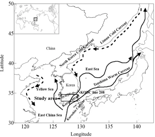
Fig. 1-1. The study area and its major currents (dotted line: cold current, solid line: warm current). ... 13 Fig. 1-2. Correspondence analysis of biomass composition of the dominant 11 species from
fisheries catches in the Korea Strait (126°-129°5'E, 33°5'-35°N) with respect to species and year from 1986 to 2010. Fig. 1-2, 1-4~5 and 1-7~10 can be overlapped for graphical interpretation. ... 17 Fig. 1-3. Species composition in biomass of the fisheries catches in the Korea Strait
(126°-129°5'E, 33°5'-35°N) from 1986 to 2010 by (a) year and (b) month. The data were provided by National Institute of Fisheries Science (NIFS). ... 18 Fig. 1-4. Correspondence analysis of biomass composition of the dominant 11 species from
fisheries catches in the Korea Strait (126°-129°5'E, 33°5'-35°N) with respect to species and bi-month from February to December. Fig. 1-2, 1-4~5 and 1-7~10 can be
overlapped for graphical interpretation. ... 19 Fig. 1-5. Correspondence analysis of biomass composition of the dominant 11 species from
fisheries catches in the Korea Strait (126°-129°5'E, 33°5'-35°N) with respect to species and fishing block. Fig. 1-2, 1-4~5 and 1-7~10 can be overlapped for graphical
interpretation. ... 20 Fig. 1-6. Classification of fishing blocks based on correspondence analysis of biomass
composition of the dominant 10 species from fisheries catches in the Korea Strait (126°-129°5'E, 33°5'-35°N) from 1986 to 2010. ... 21 Fig. 1-7. Canonical correspondence analysis on annual fish assemblage in the Korea Strait
and water temperature at 0 m depth with time lags of 0-2 yr. Oceanic conditions that were not significantly correlated at 95% confidence interval are omitted. Fig. 1-2, 1-4~5
iv
and 1-7~10 can be overlapped for graphical interpretation. ... 25 Fig. 1-8. Canonical correspondence analysis on annual fish assemblage in the Korea Strait
and water temperature at 10 m with time lags of 0-2 yr. Oceanic conditions that were not significantly correlated at 95% confidence interval are omitted. Fig. 2, 4~5 and 1-7~10 can be overlapped for graphical interpretation. ... 25 Fig. 1-9. Canonical correspondence analysis on annual fish assemblage in the Korea Strait
and water temperature at 20 m depth with time lags of 0-2 yr. Oceanic conditions that were not significantly correlated at 95% confidence interval are omitted. Fig. 1-2, 1-4~5 and 1-7~10 can be overlapped for graphical interpretation. ... 26 Fig. 1-10. Canonical correspondence analysis on annual fish assemblage in the Korea Strait
and the inflow index of KSBCW and bottom salinity at 125-m depth with time lags of 0-2 yr. Oceanic conditions that were not significantly correlated at 95% confidence interval are omitted. Fig. 1-2, 1-4~5 and 1-7~10 can be overlapped for graphical
interpretation. ... 26 Fig. 1-11. Annual inflow index of the Korea Strait Bottom Cold Water estimated in the
KODC line 208 from 1986 to 2010 (black line). The red line represents the step changes detected. ... 29 Fig. 1-12. Annually-averaged water temperature at (a) 0, (b) 10 and (c) 20 m depths in the
Korea Strait from 1986 to 2010. The red line represents the step changes detected. ... 30 Fig. 1-13. Annually-averaged salinity at 125-m depth in the Korea Strait from 1986 to 2010.
The red line represents the step changes detected... 31 Fig. 2-1. Estimated daily spawning fraction rate of Pacific anchovy Engraulis japonicus in
the Korea Strait. ... 61 Fig. 2-2. Yield per recruit of Pacific anchovy Engraulis japonicus with varying instantaneous fishing mortality and varying (a) minimum fork length of allowed catch (smaller fish are
v
protected and bigger fish are allowed for commercial catch); (b) maximum fork length of allowed catch (bigger fish are protected and smaller fish are allowed for commercial catch). ... 68 Fig. 2-3. Yield per recruit curves of Pacific anchovy Engraulis japonicus with varying
instantaneous fishing mortality when (a) minimum fork length of allowed catch=30 mm; (b) maximum fork length of allowed catch=30 mm. F0.1 is a reference point of
instantaneous fishing mortality where the slope of the yield per recruit curve
corresponds to 10% of the initial slope at the origin and Y0.1 is the corresponding catch;
Fmax is a reference point of instantaneous fishing mortality where the slope of the yield
per recruit curve equals zero and Ymax is the corresponding catch. ... 69
Fig. 2-4. Egg production per recruit of Pacific anchovy Engraulis japonicus with varying instantaneous fishing mortality and varying (a) minimum fork length of allowed catch (smaller fish are protected and bigger fish are allowed for commercial catch), (b) maximum fork length of allowed catch (bigger fish are protected and smaller fish are allowed for commercial catch)... 71 Fig. 3-1. Yield per recruit of chub mackerel Scomber japonicus with the varying length at
first capture (Lc) and instantaneous fishing mortality (F) when water temperature is
assumed to be 20℃ for the growth during the larval stage (< 1.5 cm in standard length). ... 95 Fig. 3-2. Yield per recruit curve of chub mackerel Scomber japonicus varying with the length
at first capture (Lc=15, 20, 25, 30 cm) and the corresponding values of F0.1. F0.1 is the
value of F at which the corresponding slope of yield-per-recruit curve equals to the 10% of the initial slope at the origin (F = 0). ... 96 Fig. 3-3. Yield-per-recruits of chub mackerel Scomber japonicus at the reported fishing
vi
15 to 30 cm in fork length. Ymax is the maximum yield. ... 97
Fig. 3-4. Yield of chub mackerel Scomber japonicus with varying water temperature and instantaneous fishing mortality (F). when the length at first capture=15 cm and the maximum length of the larva, whose growth is assumed temperature-dependent, is assumed to be 1.5 cm. ... 99 Fig. 3-5. Yield (Y0.1 and Ymax) of chub mackerel Scomber japonicus with varying water
temperature. Y0.1 and Ymax are the yields corresponding to the instantaneous fishing
mortality (F) are F0.1 and Fmax. F0.1 is the value of F at which the corresponding slope of
yield-per-recruit curve equals to the 10% of the initial slope at the origin (F=0). Fmax is
the value of F at which the yield-per-recruit is maximized. ... 100 Fig A-1. Flower chart of yield-per-recruit analysis of anchovy. ... 113
vii
List of tables
Table 1-1. Correlation coefficient of the monthly water temperature and salinity, averaged over the water column up to 120-m depth at the stations along the KODC 208 line with respect to the bimonthly total catch in the Korea Strait from 1986 to 2010. The values in underline demote p<0.05. ... 23 Table 1-2. Correlation coefficients between the first dimension from correspondence analysis
and the environmental variables with time lags of 0-2 yr. The coefficients in underline denote p<0.05 (TWC: Inflow index of Tsushima Warm Current, KSBCW: Inflow index of Korea Strait Bottom Cold Water, T: water temperature, S: salinity, 0-125: depth in meter) ... 24 Table 1-3. Cross-correlation coefficients of the annual catch of fish species in the Korea
Strait with the inflow index of the Korea Strait Bottom Cold Water (KSBCW), depth-specific water temperature (T) and salinity (S) at the KODC 208-4 station from 1986 to 2010. The coefficients of underline denote p<0.05, and the number in parenthesis denote the time lag in year. The digits 0-125 denote depth in meter. ... 34 Table 1-4. Reported start year of shift in fish assemblage structure by region in the Korean
waters from 1986 to 2010 ... 36 Table 3-1. Variation of F0.1, Fmax and Lc,max with respect to varying water temperature
condition (15, 17, 18, 23℃) during the early life stages of chub mackerel Scomber
japonicas. F0.1 is the instantaneous fishing mortality (F) at which the corresponding
slope of yield-per-recruit curve equals to the 10% of the initial slope at the origin (F=0).
Fmax is the value of F at which the yield-per-recruit is maximized. Lc is the fork length at
first capture and Lc,max is the value of Lc at which the yield-per-recruit is maximized
viii
Abstract
This study showed 1) the multi-decadal changes in fish assemblages in relation to oceanic environment change in the Korea Strait, and 2) biological reference points and current fishing level for sustainable fisheries of Pacific anchovy and chub mackerel representing the dominant species in the Korea Strait.
Chapter 1, I evaluated spatio-temporal changes of the fish-assemblage structure in the Korea Strait (KS, 126°-129°5'E, 33°5'-35°N) and its relationship with oceanic conditions from 1986 to 2010. Hydrographic data include depth-specific water temperature, salinity and inflow indices of the Tsushima Warm Current (TWC) and Korea Strait Bottom Cold Water (KSBCW). Spatio-temporal changes of the fish-assemblage structure and relationship with oceanic conditions evaluated by Correspondence analysis (CA) and canonical
correspondence analysis (CCA). Anchovy was the most dominant species in the KS from 1986 to 2010. Shift in the fish assemblage was detected between 1990 and 1991. Sardine and filefish dominated from 1986 to the early-1990s, and chub mackerel and squid dominated from the early-1990s to 2010. Annual changes in fish assemblages were significantly correlated surface water temperature at 0-20 m depths. Regime shift in surface water temperature was detected shift in 1987. Among the significant oceanic conditions, water temperature delayed by 1 year showed the most significant correlation with change in fish assemblage structure. I conclude that 1) fish assemblage structure dramatically shift in the 1990-1991, 2) the KS is an intermediate area between the waters off Ieodo and the East Sea with respect to the timing of shift in fish assemblage structure, 3) the shift of fish assemblage structure in the KS was highly influenced by climate shift of surface water temperature in the late-1980s.
ix
Chapter 2, I developed and applied a simulation-based yield-per-recruit analysis that considered temperature-dependent growth and size-dependent mortality from egg to adult stages of anchovy. I projected changes in fisheries yield and egg production of anchovy with respect to varying biological reference points of 1) the instantaneous fishing mortality (F), 2) the minimum fork length of anchovy allowed to catch for protecting smaller anchovy (Lc,min),
and 3) the maximum fork length allowed to catch for protecting bigger anchovy (Lc,max).
Simulation showed that the anchovy yield will be maximized at ca. 1.4×10⁶ tons when Lc,min
ranges between 42-60 mm or at ca. 0.8×10⁶ tons when Lc,max ranges from 88-160 mm. At
Lc,min=30 mm, the present minimum length of catch, simulation indicated that the anchovy
yield can reach a maximum of 1.3×10⁶ tons in the long-term when F0.1=0.028 day -1
. I expect that this yield-per-recruit model can be applied to other commercially-important small pelagic species in which the traditional Beverton-Holt Y/R model is difficult to apply.
Chapter 3, to provide the biological reference points for management of chub mackerel stock, I applied a simulation-based yield-per-recruit analysis that considered 1) temperature-dependent growth in early life stage, 2) size-dependent mortality. I estimated fisheries yield with respect to varying biological reference points and environmental conditions such as 1) the instantaneous fishing mortality (F), 2) the length at first capture (Lc), and 3) spawning water temperature. The result of simulation showed that the
yield-per-recruit (Y/R) could be greater when the Lc ranges from 19-27 cm and F ranges from 1.48-2
yr-1. Y/R with respect to varying spawning water temperature from 15 to 23℃ showed an increasing trend with increasing temperature. I suggest targeting an Lc of 17 cm (age=0.6
years) at F=0.48 yr-1, which is the current fishing mortality, for maximizing the chub mackerel harvest.
1
General introduction
Global fisheries
Global fishery production was 16.7 million tons (86% of total world fish production) in 1950. It increased dramatically to 87.7 million tons in 1996, and then declining to stabilize at about 80 million tons (FAO, 2011). Global fishery production was 82.6 million tons in 2011 and 79.7 million tons in 2012. In these years, the Northwest Pacific had the highest production with 26% of the global fishery production, followed by the Southeast Pacific (15%), the Western Central Pacific (14%) and the Northeast Atlantic (9%) (FAO, 2014). Especially the Pacific and Atlantic Oceans, where showed high fishery production and consumption, require establishment of fisheries resource management plan (Zhang and Kim, 1996).
Korean fisheries
Total catch in Korean coastal waters averaged 1.25 million tons from 1970 to 2018. Catch began to increase from 0.72 million tons in 1970, the largest catch of 1.73 million tons occurred in 1986. After that it steadily decreased until recent year (MOF, 2020). Fishery production in Korean waters steadily decreased, and trophic levels meaning ecosystem structure also decreased with decreasing fishery production (Zhang, 2006). The Korean coastal waters are divided into the three regions, 1) the East Sea, 2) the Korea Strait and 3) the Yellow Sea. Catch of coastal fisheries in the Yellow Sea from 1990 to 2010 showed the highest catch (71,000 tons) before late-2000s. Since late-2000s, the Korea Strait (81,218 tons) showed the highest catch compare with other seas (Yoon et al., 2014).
2
Cause of changes in fisheries resources
Distribution and abundance of pelagic and demersal fish species are known as influenced by climate change (Gong et al., 2007; Gong et al., 2010; Perry et al., 2005; Reid et al., 2001; Tian et al., 2011). Overfishing also is known to affect changes in fisheries resource together with climate change (Kim et al., 2007). In Korean waters, it is difficult to estimate the total biomass by species because various fish species inhabit with together (Zhang and Kim, 1996). Thus, studies on evaluating 1) the long-term change in fish
assemblage and 2) the current fishing level by fish species are needed to determine whether climatic change or fishery was the major cause of the variation in fishery production in Korean waters.
Summary
This study evaluated 1) long-term changes in fish assemblages in relation to climate change in the Korea Strait, and 2) biological reference points for suitable fisheries
management of anchovy and chub mackerel representing the dominant species in the Korea Strait.
Long-term changes in fish assemblages in the Korea Strait
In Chapter 1, I evaluated long-term changes in fish assembles in the Korea Strait. The Korea Strait is a mixed area of the Korea Strait Bottom Cold Water (KSBCW) flowing southward and the Tsushima Warm Current (TWC) flowing northward. The Korea Strait is commercially important area because 1) fisheries production was the highest among the
3
Korean waters from late-2000s and 2) small pelagic species with high consumption are widely distributed.I estimated spatio-temporal changes in fish assemblage structure by applying CA, and relationship with changes in oceanic conditions by applying CCA.
Yield-per-recruit analysis of anchovy
In Chapter 2, I evaluated the yield-per-recruit of anchovy. Yield-per-recruit analysis diagnosis the fisheries stock and suggest biological reference points for sustainable use of fishery resources. However, traditional method of the Beverton and Holt method is difficult to apply to anchovy because of biological characteristics of anchovy. Thus, I estimated and compared the commercial yield by simulation considered the biological characteristics of anchovy at the two fishing conditions of 1) the minimum length allowed to catch and 2) the maximum length allowed to catch.
Yield-per-recruit analysis of chub mackerel
In Chapter 3, I evaluated the yield-per-recruit of chub mackerel. Growth rate of fish is the most high in early life stage and is affected by changes in water temperature. Thus, I applied a simulation-based yield-per-recruit model that considered 1) temperature-dependent growth in early life stage, 2) size-dependent mortality. I evaluated fisheries yield with respect to varying biological reference points and environmental conditions, including 1) the instantaneous fishing mortality (F), 2) the length at first capture (Lc), and 3) water
4
References
FAO. 2011. Review of the state of world marine fishery resources. Food and agriculture organization of the United Nations, Rome, Italy, 142-145.
FAO. 2014. The State of World Fisheries and Aquaculture 2014: Opportunities and
challenges. Food and agriculture organization of the United Nations, Rome, Italy, 37-37. Gong Y, Suh Y, Seong K and Han I. 2010. Climate change and marine ecosystem. Academy
Book press, Seoul, Korea, 45, 181-186.
Gong Y, Jeong HD, Suh YS, Park JH, Seong KT, Kim SW, Choi KH and Han IS. 2007. Fluctuations of pelagic fish populations in relation to the climate shifts in the Far-East regions. J Ecol Field Biol 30, 23-38. https://doi.org/10.5141/JEFB.2007.30.1.023. Kim S, Zhang CI, Kim JY, Oh JH, Kang S and Lee JB. 2007. Climate variability and its
effects on major fisheries in Korea. Ocean Sci J 42, 179-192. https://doi.org/10.1007/BF03020922.
MOF (Ministry of Oceans and Fisheries). 2020. Fisheries information service (1970-2018). Retrieved from http://www.mof.go.kr/stat Portal on 24 July 2020.
Perry AL, Low PJ, Ellis JR and Reynolds JD. 2005. Climate change and distribution shifts in marine fishes. Science 308, 1912-1915. 10.1126/science.1111322.
Reid PC, de Fatima Borges M and Svendsen E. 2001. A regime shift in the North Sea circa 1988 linked to changes in the North Sea horse mackerel fishery. Fish Res 50, 163-171. https://doi.org/10.1016/S0165-7836(00)00249-6.
5
Tian Y, Kidokoro H and Fujino T. 2011. Interannual-decadal variability of demersal fish assemblages in the Tsushima Warm Current region of the Japan Sea: Impacts of climate regime shifts and trawl fisheries with implications for ecosystem-based management. Fish Res 112, 140-153. https://doi.org/10.1016/j.fishres.2011.01.034.
Yoon SC, Jeong YK, Zhang CI, Yang JH, Choi KH and Lee DW. 2014. Characteristics of Korean coastal fisheries. Kor J Fish Aquat Sci 47, 1037-1054.
http://dx.doi.org/10.5657/KFAS.2014.1037.
Zhang CI and Kim S. 1996. Consideration on the management of fisheries resources under the EEZ regime. Ocean Policy Research, 179-198.
Zhang CI. 2006. A study on the ecosystem-based management system for fisheries resources in Korea, J Kor Soc fish Tech, 42(2), 179-198.
6
Chapter 1
Long-term changes in dominant fish species and relationship with
climate change in the Korea Strait from 1986 to 2010
Abstract
I evaluated the spatio-temporal changes in fish assemblages, and its relationship with oceanic conditions in the Korea Strait (KS, 126°-129°5'E, 33°5'-35°N) from 1986 to 2010. I used the inflow indices of the Korea Strait Bottom Cold Water (KSBCW) and the Tsushima Warm Current (TWC), water temperature and salinity data from 1986 to 2010.
Correspondence analysis (CA) detected a shift in the fish assemblage between 1990 and 1991. Sardine and filefish were dominant species from 1986 to 1990, and thereafter chub mackerel and squid became dominant. Surface temperatures at 0-20 m depths, especially with a time lag of 1 yr, were significantly correlated with the 1990-1991 shift in fish assemblage structure. I hope that further multidisciplinary studies between regional oceanographers and fisheries scientists will contribute to development of fisheries policies by understanding interactions between oceanographic processes and fishes at the regional scale in adaptation to climate change.
Key words: correspondence analysis; canonical correspondence analysis; climate change; fish assemblage; regime shift
7
Introduction
Climate change and regime shift in the North Pacific
A regime shift is a large, decadal-scale switch in the structure of the marine
ecosystem, which is associated with changes in the climate systems (Beaugrand, 2004; Reid et al., 2001; Rodionov and Overland, 2005). In the North Pacific, climate regime shifts were reported to have occurred in 1976/1977, 1988/1989 and 1998/1999 (Hare and Mantua, 2000; Minobe, 2000; Overland et al., 2008; Watanabe et al., 2005). Among various climate indices, the Pacific Decadal Oscillation and the Artic Oscillation were particularly related with the shifts (Chiba et al., 2006; Mantua et al., 1997; Rodionov and Overland, 2005).
Impacts of climate change on marine fishes
Climate change affects the biology, recruitment, spatial distribution, migration and human exploitation of marine fishes (Drinkwater, 2005; Kell et al., 2005; Lehodey et al., 2006). Many small pelagic species such as sardine (Sardinops sagax), anchovy (Engraulis
japonicus) and chub mackerel (Scomber japonicus) have a direct relationship with climate
regime shift (Gong et al., 2007; Gong et al., 2010; Reid et al., 2001). These environmental changes also effect on distribution and abundance of demersal species inhabiting deep waters of more than 200 m such as Pacific cod (Gadus macrocephalus) and flathead flounder (Hippoglossoides dubius) (Perry et al., 2005; Tian et al., 2011; Tu et al., 2015). Among these, demersal or less mobile species are more vulnerable to changes in the marine environment than short-live pelagic and cephalopods, because 1) they have been adapted to relatively stable environment, and 2) have limitation in migration to suitable habitat for growth and spawning (Yatsu et al., 2013).
8
Korea Strait (KS)
The Korea Strait (KS) is located southward of Korea, and connects the East China Sea and the East Sea. The KS is approximately 280-km length and 200-km wide with depths up to 150 m (Cho and Kim, 1999; Yi, 1966).
The major currents in the KS
The Tsushima Warm Current (TWC) and the Korea Strait Bottom Cold Water (KSBCW) are major currents in the KS (Na et al., 2010). The TWC, a branch of the Kuroshio, flows northeastward from west of Kyushu into the southern portion of the East Sea through the upper layer, and the KSBCW flows southwestward from the East Sea into the KS through the bottom layer (Na et al., 2010; Yi, 1996).
The Tsushima Warm Current (TWC)
The TWC transports high-temperature water and fish larvae from the East China Sea into the East Sea through the KS (Beardsley et al., 1985; Hsueh et al., 1996; Isobe, 1999; Isobe et al., 1994; Lie and Cho, 1994; Lim and Chang, 1969; Na et al., 2010; Yi, 1966). The TWC is divided into two branches at the KS, one branch flows to the East Sea and another branch flows to the Japanese northern coast (Cho and Kim, 1999). Surface-current speed of the TWC exceeds 80 cm s-1 near the Korean coast and 40 cm s-1 near the Japanese coast, and the total volume transport is high in summer and autumn and low in winter and spring (Isobe et al., 1994).
9
The Korea Strait Bottom Cold Water (KSBCW)
The Korea Strait Bottom Cold Water originated from the deeper East Sea (Cho and Kim, 1998; Na et al., 2010; Sudo, 1986). It flows near the shallow within 50 km and shows seasonal variations in the volume transport (Cho and Kim, 1998). Its temperatures are below 10°C and salinities range from 34.0-34.4 (Lim and Chang, 1969; Na et al., 2010). The cold water of the KSBCW appears in the KS from Jun to February and the bottom temperature becomes lowest in August (Lim and Chang, 1969).
Ecology in the KS
Primary productivity and phytoplankton
In the KS, the nutrients for phytoplankton are supplied from the bottom layer to the mixed layer by physical processes such as the TWC in spring and typhoon in summer and autumn (Chang et al., 1996; Gong et al., 1996; Jang et al., 2013; Shiah et al., 2000). Primary productivity in the western channel of the KS is higher in spring (3.42-6.68 mg C m-3 h-1) and autumn (9.24-13.05 mg C m-3 h-1) than in summer (0.57-0.79 mg C m-3 h-1) and winter (0.75-1.77 mg C m-3 h-1) (Chin and Hong, 1985). The annual phytoplankton species composition depends on thermohaline structures which is largely divided into mixed periods (December-May) and stratified periods (Jun-November). Diatoms dominate during the mixed periods while nanoplankton group dominate during the stratified periods (Shon et al., 2008).
10
Zooplankton
Zooplankton transfer energy between producer and consumer in the ocean (Jang et al., 2012). In the KS, the species diversity of zooplankton increased from spring to autumn and decreased from autumn to winter (Moon et al., 2010). Copepods are the most abundant, but their dominance tend to decrease with increasing abundance of salps (Jang et al., 2012; Kang et al., 2019), which compete for phytoplankton food with copepods and fish larvae (Kang et al., 2000; Kashkina, 1986).
Fish
Small pelagic fish species such as anchovy, Pacific sardine, chub mackerel and common squid dominate the fisheries catches from the KS (Kim and Kang, 2000). Many small pelagic fish use the KS as a migration route between the East China Sea and the East Sea as well as spawning and nursery grounds (Kim, 2003). In addition, filefish
(Thamnaconus modestus), hairtail (Trichiurus lepturus), Pacific cod and yellow croaker (Larimichthys polyactis) are major demersal fishes harvested in the KS (Jung et al., 2013c; Chung et al., 2013). The changes in the distribution and catch of fish in the KS were mostly explained by variation of surface and bottom water temperature in relation with the regime shifts in the North Pacific (Beamish, 2008; Jung et al., 2013c).
11
Past studies on impact of climate change and regime shift of commercial fish
assemblage in Korean waters
Past studies evaluated and related long-term changes in the composition and
distribution of fisheries species in the adjacent seas of Korea with climate change. Kim and Kang (2000) documented the change in the physical environments during the past 30 years in the KS and its impact on the low and high trophic levels. Gong et al. (2007) and Kim et al. (2007) studied the relationship between climate/environmental variables such as climate regime shift, El Niño and responses of major fisheries species in the adjacent seas of Korea. Jung et al. (2013c) reported latitudinal shifts of major fisheries species in relation to
fluctuations of water temperature, salinity and dissolved oxygen in Korean Waters. Hwang and Jung (2012), Jung et al. (2013b) and Jung (2014) evaluated multi-decadal changes in composition of major fisheries species in relation to fluctuations of ocean environmental factors in the adjacent seas of Korea.
Problems
Despite the KS showed highest fisheries production compared with the adjacent seas of Korea from late 2000s, studies on changes in fish community of pelagic and demersal fisheries species related with climate change are in shortage. Most of the studies regarding fish assemblage have been conducted in the inshore waters of the KS without utilization of the data of commercial fisheries catch from the offshore waters (Cha et al., 2007; Huh and Kwak, 1998; Jeong et al., 2013; Kim et al., 2000; Kim et al., 2003a, Kim et al., 2003b; Kim and Gwak, 2006; Kwak et al., 2008). In addition, studies on regional changes of fish assemblages were conducted in the adjacent seas of Korea, but regional comparisons of the
12
changes have not yet conducted.
Goal and objectives
I evaluated the long-term shifts of fish assemblage structure in relation with changes in oceanic conditions in the KS driven by the regime shifts in the North Pacific to provide scientific basis in developing fisheries policies for adaptation to climate change and global warming. For this purpose, I also evaluated changes and shifts in the oceanography and fisheries assemblages of the KS to be compared with the other adjacent seas of Korea.
Data and methods
Hydrographic data
To evaluate annual changes in oceanic conditions in the KS (126°-129°5'E, 33°5'-35°N), I used the inflow indices of the TWC and the KSBCW, water temperature and salinity data from 1986 to 2010 (Fig. 1-1). I utilized the data of the inflow index values of the TWC and KSBCW provide by Na et al. (2010), and the data of water temperature and salinity provided by the Korea Oceanographic Data Center (KODC,
http://www.nifs.go.kr/kodc/soo_list.kodc) that has compiled the survey data from the bimonthly cruises conducted by the National Institute of Fisheries Science (NIFS).
The KODC line 208 was selected to evaluate the annual changes of water
temperature and salinity at the depths ranging from 0 to 125 m in the KS, because the inflow indices of the TWC and the KSBCW were also calculated based on the data from the line
13
208 (Jung et al., 2013b; Na et al., 2010). I excluded the December data for all years to avoid unbiased evaluation, because the cruise survey was not conducted in December of 1991 and 1992.
Fig. 1-1. The study area and its major currents (dotted line: cold current, solid line: warm current).
14
Fisheries data
To evaluate long-term changes in fish assemblages in the KS, I used monthly
commercial fisheries catch data from 1986 to 2010 provided by NIFS. The data composed 1) year, 2) month, 3) fishing location (fishing block with latitude and longitude) and 4) catch (kg in wet weight). I evaluated the spatial and temporal variations of fish assemblage structure based on the biomass composition of catch by fish species. I aggregated the monthly catch data to bimonthly data to be compatible with the bimonthly KODC data.
Analyses
Detection of oceanic regime shift in the KS
To detect temporal shifts in the oceanic conditions of the KS, I applied a sequential t-test of regime shift (STARS) developed by Rodionov (2004) to the annual time series of the depth-specific water temperature and salinity and the inflow indices of the two major currents. A regime shift in STARS was defined by the following three criteria: 1)
significance level, 2) cut-off length (L) and 3) Huber’s weight parameter (H). Significance level is the probability of Type I error. Cut-off length (L) is the minimum time length of the regimes and Huber’s weight parameter (H) acts as controlling the weighting value assigned to the outliers. More detailed descriptions are explained at www.beringclimate.noaa.gov (Keevallik, 2011; Rodionov, 2006). To detect at least one shift of all oceanic conditions and consider all outliers, I set significance level=0.3 and H=1. I set L=7.5 because the velocity and discharge of the Kuroshio Current showed long-term cycle of 6-9 years (Gong et al., 2010; Miita and Tawara, 1984).
15
Changes in fish assemblages and its relationship with oceanic conditions
Commercial fisheries catch data comprised a total of 137 fish species. I selected the top-10 dominant species in total catch which occupied more than 1% in the total catch from 1986 to 2010. I aggregated the remaining species into a single category (’others’) to
summarize annual, monthly and spatial changes of the dominant fish species in the KS. To evaluate spatio-temporal changes of the fish-assemblage structure in the KS by three categorical variables 1) year, 2) month, and 3) fishing block, I graphically summarized the species compositions in biomass of the commercial fisheries catch data by
correspondence analysis (CA) from 1986 to 2010 (Hwang and Jung, 2012; Ter Braak, 1986). I calculated the correlation coefficients between the averaged environmental factors using the water column at each station and the sum of total catch for bimonthly in each year from 1986 to 2010 in the KS. Then, I selected the two stations where the correlation
coefficient was the most significant for water temperature and salinity. Additionally, I calculated the cross-correlation coefficients with the time lags of 1 and 2 years for each station to evaluate possible delayed effects of the environmental variables on the fish assemblage structure.
I correlated the first and second dimensions extracted from our CA with the
environmental variables (annually averaged depth-specific water temperature and salinity at the selected two stations and the annual inflow of the TWC and the KSBCW) to apply canonical correspondence analysis (CCA) (Ter Braak, 1986). I selected the environmental variables whose correlation coefficient was significant with respect to the first or the second dimension to be shown in the CCA graphics. The CA and CCA were run by the “vegan” package in the R software (3.6.3) (Oksanen, 2018).
16
Results and discussion
Temporal variability and spatial distribution of fish assemblage structure
Annual change
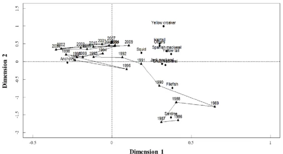
My CA showed that fish assemblage in the KS dramatically shifted in 1990-1991, and thereafter it was stabilized from 1993 to 2010 (Fig. 1-2). The variability of species biomass composition in fish assemblage during 1986-2010 was mostly explained by two dimensions (44.19% and 21.93%).
From 1986 to 1990, anchovy (36.62%) was the most dominant, followed by sardine (17.67%), filefish (16.04%), chub mackerel (11.24%) and hairtail (5.65%) (Fig. 1-3, a). The dominant fish species from 1991 to 2010 were anchovy (55.8%), chub mackerel (10.53%), squid (7.61%) and hairtail (6.3%) (Fig. 1-3, a).
17
Fig. 1-2. Correspondence analysis of biomass composition of the dominant 11 species from fisheries catches in the Korea Strait (126°-129°5'E, 33°5'-35°N) with respect to species and year from 1986 to 2010. Fig. 1-2, 1-4~5 and 1-7~10 can be overlapped for graphical interpretation.
18
Fig. 1-3. Species composition in biomass of the fisheries catches in the Korea Strait (126°-129°5'E, 33°5'-35°N) from 1986 to 2010 by (a) year and (b) month. The data were provided by National Institute of Fisheries Science (NIFS).
19
Monthly change
My CA divided the monthly compositions of species biomass into three seasonal groups; 1) Spring (from April to Jun), 2) Summer (August) and 3) Autumn-Winter (from October to February) (Fig. 1-4). The dominant species were anchovy (37.26%), sardine (15.68%), chub mackerel (13.39%) and filefish (8.78%) in spring; anchovy (77.26%) and chub mackerel (8.81%) in summer; anchovy (48.71%), squid (10.53%), chub mackerel (10.38%) and hairtail (7.86%) in autumn-winter (Fig. 1-3, b). Anchovy, sardine, squid and filefish particularly showed greater seasonal variability.
Fig. 1-4. Correspondence analysis of biomass composition of the dominant 11 species from fisheries catches in the Korea Strait (126°-129°5'E, 33°5'-35°N) with respect to species and bi-month from February to December. Fig. 1-2, 1-4~5 and 1-7~10 can be overlapped for graphical interpretation.
20
Spatial distribution in fish assemblage
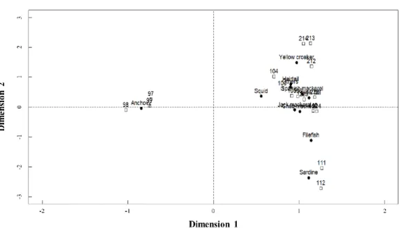
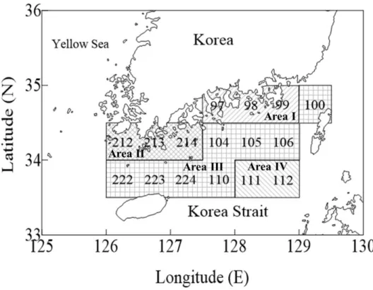
I could the entire study area into 4 Areas based on the similarity in species
composition summarized by my CA (Fig. 1-5). Anchovy mainly distributed in Area Ⅰ. Yellow croaker mainly distributed in Area Ⅱ. Squid, jack mackerel and Spanish mackerel mainly distributed in Area Ⅲ. Sardine and filefish mainly distributed in Area Ⅳ. Chub mackerel mainly distributed in Area Ⅲ and Ⅳ, and hairtail mainly distributed in Area Ⅱ and Ⅲ (Fig. 1-6).
Fig. 1-5. Correspondence analysis of biomass composition of the dominant 11 species from fisheries catches in the Korea Strait (126°-129°5'E, 33°5'-35°N) with respect to species and fishing block. Fig. 1-2, 1-4~5 and 1-7~10 can be overlapped for graphical interpretation.
21
Fig. 1-6. Classification of fishing blocks based on correspondence analysis of biomass composition of the dominant 10 species from fisheries catches in the Korea Strait (126°-129°5'E, 33°5'-35°N) from 1986 to 2010.
22
Grouping of species based on spatio-temperal variability
Sardine and filefish which dominate in spring were sharply decreased after the early-1990, and mainly distributed far away from the coast. Anchovy was mostly caught in summer in near the Southeast coast of Korea, and the annual catch of anchovy steadily increased from 1986 to 2010. Squid and hairtail dominated in autumn-winter. Squid showed high variability in annual catch compare with other species, and hairtail dramatically decreased in 1993 and then steadily increased to 2010. The two species mainly distributed from the Northern part of Jeju Island to the Southeast sea of Korea. Chub mackerel that was constant of annual and seasonal catch from 1986 to 2010, mainly distributed along with sardine, filefish, squid and haritail (Fig. 1-6). Yellow croaker, jack mackerel and Spanish mackerel showed less than 5% in total catch by season.
Impact of oceanic condition on the fish assemblage
The relationship between changes in oceanic conditions and fish assemblages
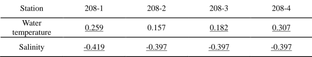
As a result of cross-correlation between changes in oceanic conditions and fish assemblages, water temperature of 208-4 station and salinity of 208-1 station showed the highest correlation with total catch. However, we applied salinity data at 208-4 station because 208-1 station is shallower than other stations and the difference in correlation coefficient was small between stations (Table 1-1).
23
Table 1-1. Correlation coefficient of the monthly water temperature and salinity, averaged over the water column up to 120-m depth at the stations along the KODC 208 line with respect to the bimonthly total catch in the Korea Strait from 1986 to 2010. The values in underline demote p<0.05.
Station 208-1 208-2 208-3 208-4 Water
temperature 0.259 0.157 0.182 0.307 Salinity -0.419 -0.397 -0.397 -0.397
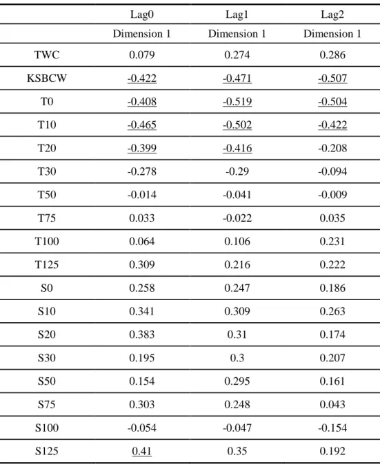
I conducted cross-correlation and CCA to evaluate the relationship between the oceanic conditions and fish assemblages. Annually-averaged index of KSBCW, surface water temperature at 0-20 m and bottom salinity at 125 m were significantly correlated with first dimension (Table 1-2 and Fig. 1-7~10). KSBCW and surface water temperature showed negative correlation with first dimension while bottom salinity showed positive correlation. Among the significant oceanic conditions, the correlation of water temperature at 10 m depth showed highest value, followed by KSBCW and salinity at 125 m.
24
Table 1-2. Correlation coefficients between the first dimension from correspondence analysis and the environmental variables with time lags of 0-2 yr. The coefficients in underline denote p<0.05 (TWC: Inflow index of Tsushima Warm Current, KSBCW: Inflow index of Korea Strait Bottom Cold Water, T: water temperature, S: salinity, 0-125: depth in meter)
Lag0 Lag1 Lag2 Dimension 1 Dimension 1 Dimension 1 TWC 0.079 0.274 0.286 KSBCW -0.422 -0.471 -0.507 T0 -0.408 -0.519 -0.504 T10 -0.465 -0.502 -0.422 T20 -0.399 -0.416 -0.208 T30 -0.278 -0.29 -0.094 T50 -0.014 -0.041 -0.009 T75 0.033 -0.022 0.035 T100 0.064 0.106 0.231 T125 0.309 0.216 0.222 S0 0.258 0.247 0.186 S10 0.341 0.309 0.263 S20 0.383 0.31 0.174 S30 0.195 0.3 0.207 S50 0.154 0.295 0.161 S75 0.303 0.248 0.043 S100 -0.054 -0.047 -0.154 S125 0.41 0.35 0.192
25
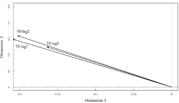
Fig. 1-7. Canonical correspondence analysis on annual fish assemblage in the Korea Strait and water temperature at 0 m depth with time lags of 0-2 yr. Oceanic conditions that were not significantly correlated at 95% confidence interval are omitted. Fig. 2, 4~5 and 1-7~10 can be overlapped for graphical interpretation.
Fig. 1-8. Canonical correspondence analysis on annual fish assemblage in the Korea Strait and water temperature at 10 m with time lags of 0-2 yr. Oceanic conditions that were not significantly correlated at 95% confidence interval are omitted. Fig. 1-2, 1-4~5 and 1-7~10 can be overlapped for graphical interpretation.
26
Fig. 1-9. Canonical correspondence analysis on annual fish assemblage in the Korea Strait and water temperature at 20 m depth with time lags of 0-2 yr. Oceanic conditions that were not significantly correlated at 95% confidence interval are omitted. Fig. 2, 4~5 and 1-7~10 can be overlapped for graphical interpretation.
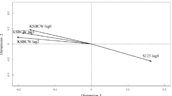
Fig. 1-10. Canonical correspondence analysis on annual fish assemblage in the Korea Strait and the inflow index of KSBCW and bottom salinity at 125-m depth with time lags of 0-2 yr. Oceanic conditions that were not significantly correlated at 95% confidence interval are omitted. Fig. 1-2, 1-4~5 and 1-7~10 can be overlapped for graphical interpretation.
27
Relationship between changes in oceanic conditions and fish assemblage
structure with varying time lags
Cross-correlation and CCA showed the influences of changing oceanic conditions on fish assemblage structure varied by time lags. Fluctuations of the KSBCW before 2 years and surface water temperature before 1 year showed the most significant correlation with annual changes in fish assemblages (Table 1-2, Fig. 1-7~10). Salinity showed the most significant correlation with fish assemblages at the same time (time lag0) (Table 2, Fig. 1-10).
Cause of the most significant correlation between catch by fish species and
one-year delayed surface water temperature
Correlation coefficients between annual catch of the dominant species with the annual-averaged surface water temperatures at 0-20 water depths were the most significant at a time lag of 1 yr. This can be explained by the three factors: 1) The mean age at first catch was 1 yr, 2) the fish species spend their early-life stages (egg and larval stages) in the surface layer of the KS (Choi et al., 2004; Hwang et al., 2006; Jung, 2008a; Jung et al., 2013a; Kramer, 1960; Lee et al., 2013; Sassa and Konishi, 2006; Zhang, 1996; Zhang and Lee, 2001), and 3) variability in temperature-dependent growth and mortality during the early-life stages is critical in determining the subsequent recruitment levels (Go et al., 2020; Houde, 1989; Jung et al., 2008).
28
Hydrography
I selected only the environmental factors that showed significant correlations with the two dimensions of our CA to evaluate long-term changes in oceanic conditions and their influences on the fish assemblage structure in the KS.
Annual inflow index of the KSBCW showed three regime shifts during 1986-2010 (Fig. 1-11). The inflow index of the KSBCW showed decreasing shift in 1986-1987 and maintained low values form 1987 to 1992. A shift to higher value was detected in 1993 and decreased again in 2001.
Water temperatures at 0-20 m depths steadily increased from 1986 to 2010 with a increasing shift in 1986-1987 and were particularly high in 1990 (Fig. 1-12), which was also reported in the past studies (Hwang and Jung, 2012; Jung, 2008b; Jung et al., 2013c). Additional increasing shift was detected at 0 and 10 m depths in 1996 and 1997. We speculate that the unexpected increase in water temperatures at 0 and 10 m depths in 1990 was the start of the warming trend of the surface layer in the KS.
Salinity at 125 m depth showed a decreasing shift in 1998 (Fig. 1-13). The KSBCW showed an increasing shift in the 1992-1993 with an increasing trend from 1989 to 1996.
29
Fig. 1-11. Annual inflow index of the Korea Strait Bottom Cold Water estimated in the KODC line 208 from 1986 to 2010 (black line). The red line represents the step changes detected.
30
Fig. 1-12. Annually-averaged water temperature at (a) 0, (b) 10 and (c) 20 m depths in the Korea Strait from 1986 to 2010. The red line represents the step changes detected.
31
Fig. 1-13. Annually-averaged salinity at 125-m depth in the Korea Strait from 1986 to 2010. The red line represents the step changes detected.
32
Changes in oceanic conditions and fish assemblages in the late-1980s
Thus, I speculated that the 1990-1991 shift of fish assemblage structure in the KS was triggered by the 1986-1987 shift in surface water temperature. The subsequent shift in the 1992-1993 shift in the KSBCW was followed by the 1997-1998 shift in bottom layer salinity. On the other hand, Jung (2014) and Na et al. (2010) reported that the shift of the dominant species in the southwestern East Sea in the late-1980s were influenced by the cooling of the bottom water and the warming of the surface water caused by the extending the KSBCW. The relationships between the oceanic conditions of surface and bottom layer in the KS related with the TWC and KSBCW require further oceanographic studies.
Correlation between environmental fluctuations by depth and fish species
After selecting the time lag with which the correlation was the most significant, we conducted cross-correlation analyses between the environment variables and annual catches of the dominant fish species.
Annual catch of anchovy in the KS was positively correlated with the inflow index of the KSBCW and water temperature at 0-10 m depths, and negatively correlated with salinity at 125 m depth. Catch of sardine was negatively correlated with water temperature at 0-10 m depths, and positively with salinity at 125 m depth (Table 1-3). Catches of anchovy and sardine showed an opposite trend with respect to changes in water temperature, salinity and KSBCW. Annual catches of hairtail, Spanish mackerel and yellowtail were positively correlated with surface water temperatures at 0-20 m depths. Catches of filefish were negatively correlated with water temperatures at 0-10 m depths. Catches of yellow croaker were positively correlated with water temperature at 0-10 m depths while they showed
33
negative correlations with salinity at 125 m depth. Chub mackerel, squid and jack mackerel did not show significant correlations with water temperature and salinity (Table 1-3).
34
Table 1-3. Cross-correlation coefficients of the annual catch of fish species in the Korea Strait with the inflow index of the Korea Strait Bottom Cold Water (KSBCW), depth-specific water temperature (T) and salinity (S) at the KODC 208-4 station from 1986 to 2010. The coefficients of underline denote p<0.05, and the number in parenthesis denote the time lag in year. The digits 0-125 denote depth in meter.
Anchovy Chub
mackerel Squid Hairtail Sardine Filefish
Jack mackerel Spanish mackerel Yellow croaker Yellowtail KSBCW (2) 0.475 -0.108 -0.254 -0.318 -0.166 -0.301 -0.361 0.161 0.042 0.281 T0 (1) 0.484 -0.087 0.093 0.258 -0.609 -0.448 -0.234 0.441 0.409 0.408 T10 (1) 0.496 -0.039 0.099 0.426 -0.694 -0.51 -0.108 0.65 0.532 0.39 T20 (1) 0.317 -0.155 0.112 0.203 -0.501 -0.336 0.017 0.499 0.395 0.203 S125 (0) -0.522 0.076 -0.281 -0.23 0.413 0.325 0.346 -0.276 -0.435 -0.382
35
Comparison of annual changes in dominant fish species in the KS with other
seas, the East Sea and the Northern East China Sea
I compared dominant fish species in the KS with past studies in the adjacent seas of Korea from 1980s to 2010. I could identify two groups of representative fish species in the adjacent seas of Korea from the Northern East China Sea to the East Sea: Sardine and filefish from the 1980s to the early-1990s, and chub mackerel, yellow croaker and horse mackerel from the early-1990s to 2010.
Dominant species before and after regime shifts in the early-1990s in the
adjacent seas of Korea
Fish assemblage structure in the adjacent seas of Korea including the KS showed that dominant fish species dramatically shifted in the early-1990s. Table 1-4 shows the starting year of the shift in fish community structure by region from the east to west in the Korean waters, proposed by the past and the present studies with respect to the 1988-1991 regime shift (Hwang and Jung, 2012; Jung et al., 2013b; Jung, 2014). The regional comparisons indicate that the southwestern East Sea showed the earliest response to the regime shift, followed by the KS, the waters off Jeju Island and the waters of Ieodo. Detailed mechanisms explaining these delayed responses from the east to the west need further studies.
36
Table 1-4. Reported start year of shift in fish assemblage structure by region in the Korean waters from 1986 to 2010
Region East Sea Korea Strait Waters off Jeju Islnad
Waters off Ieodo Shift year 1988 1990 1990 1991
Limitations and problems
Among 85 stations in the KS, I selected environmental data at the single 208-4 station to evaluate the annual changes of water temperature and salinity. More
comprehensive methods of evaluating the spatio-temporal variability of the oceanographic conditions to represent the whole area of the KS are needed.
Climate regime shift was reported to occur three times in the North Pacific during the 1970s-1990s (Hare and Mantua, 2000; Watanabe et al., 2005). Fish assemblage in the KS was markedly changed corresponding to the increase in KSBCW and surface water
temperature in the late-1980s, but did not show a significant response to the regime shift in the late-1990s. To specifically evaluate the impact of climate change in the late-1990 to the marine ecosystems of the Korean adjacent seas, more comprehensive researches covering all of the components from primary producers to high trophic levels are required.
37
Further Studies
Several studies on long-term spatio-temporal changes in dominant fish species were conducted at regional scale in the Korean waters, but the Yellow Sea has received less attention (Hwang and Jung, 2012; Jung et al., 2013b; Jung, 2014). For sustainable fisheries management in Korea, further researches need to cover the Yellow Sea to synthesize the regional studies on spatio-temporal variability in fish assemblage structure and its response to the climate regime shift.
The 1992-1993 shift in the inflow index of the KSBCW was preceded by the 1990-1991 shift in fish assemblages and the 1986-1987 shift in the surface water temperature. I hope that regional physical oceanographers will study and explain the time-lagged
interactions between the surface temperatures and the KSBCW, which were not detailed in my present study. Multidisciplinary co-works between oceanographers and fisheries
scientists will contribute to understanding of bio-physical interactions at the regional scale in response to climate change in the Korean waters.
Conclusion
I showed that the fish assemblage structure of the KS was shifted in 1990-1991, driven by 1988-1989 regime shift in the North Pacific, which could have corresponded to the 1986-1987 shift in the surface water temperatures detected in my study. Comparisons of my results with the past regional studies in the Korean waters suggested that the KS is an intermediate area between the waters of Ieodo and the East Sea with respect to the timing of shift in fish assemblage structure (Table 1-4). The regional shifts were characterized by the replacement of dominant fish species from sardine and filefish to chub mackerel and squid.
38
References
Beamish RJ. 2008. Impacts of climate and climate change on the key species in the fisheries in the North Pacific. North Pacific Marine Science Organization (PICES), Sidney, B.C. PICES, 101-136.
Beardsley RC, Limeburner R, Yu H and Cannon GA. 1985. Discharge of the Changjiang (Yangtze river) into the East China Sea. Cont Shelf Res 4, 57-76.
https://doi.org/10.1016/0278-4343(85)90022-6.
Beaugrand G. 2004. The North Sea regime shift: Evidence, causes, mechanisms and consequences. Prog Oceanogr 60, 245-262.
https://doi.org/10.1016/j.pocean.2004.02.018.
Cha BY, Kim DK and Seo SH. 2007. Species and Abundance Variation of Fish by a Gill Net in Coastal Waters of Southern Sea, Korea, 2006. Korean J Ichthyol 19(3), 210-224. Chang J, Chung CC and Gong GC. 1996. Influences of cyclones on chlorophyll a
concentration and synechococcus abundance in a subtropical western Pacific coastal ecosystem. Mar Ecol Prog Ser 140, 199-205. 10.3354/meps140199.
Chiba S, Tadokoro K, Sugisaki H and Saino T. 2006. Effects of decadal climate change on zooplankton over the last 50 years in the western subarctic North Pacific. Glob Chang Biol 12, 907-920. 10.1111/j.1365-2486.2006.01136.x.
Chin P and Hong SY. 1985. The Primary Production of Phytoplankton in the Western Channel of the Korea Strait. J Korean Fish Soc 18,74-83.
39
Cho YK and Kim K. 1999. Branching mechanism of the Tsushima Current in the Korea Strait. J Phys Oceanogr 30, 2788-2797.
https://doi.org/10.1175/1520-0485(2000)0302.0.CO;2.
Cho YK and Kim K. 1998. Structure of the Korea Strait Bottom Cold Water and its seasonal variation in 1991. Cont Shelf Res 18, 791-804.
https://doi.org/10.1016/S0278-4343(98)00013-2.
Choi YM, Zhang CI, Lee JB, Kim JY and Cha HK. 2004. Stock assessment and management implications of chub mackerel, Scomber japonicus in Korean waters. J Korean Soc Fish Res 6, 90-100.
Chung S, Kim S and Kang S. 2013. Ecological relationship between environmental factors and Pacific cod (Gadus macrocephalus) catch in the southern East/Japan Sea. Anim Cells Syst 17, 374-382.
Drinkwater KF. 2005. The response of atlantic cod (Gadus morhua) to future climate change. ICES J Mar Sci 62, 1327-1337. https://doi.org/10.1016/j.icesjms.2005.05.015.
Go S, Lee K and Jung S. 2020. A temperature-dependent growth equation for larval chub mackerel (Scomber japonicus). Ocean Sci J 55, 157-164.
http://dx.doi.org/10.1007/s12601-020-0004-z.
Gong GC, Chen YLL and Liu KK. 1996. Chemical hydrography and chlorophyll a
distribution in the East China Sea in summer: Implications in nutrient dynamics. Cont Shelf Res 16, 1561-1590. https://doi.org/10.1016/0278-4343(96)00005-2.
40
Gong Y, Suh Y, Seong K and Han I. 2010. Climate change and marine ecosystem. Academy Book press, Seoul, Korea, 45, 181-186.
Gong Y, Jeong HD, Suh YS, Park JH, Seong KT, Kim SW, Choi KH and Han IS. 2007. Fluctuations of pelagic fish populations in relation to the climate shifts in the Far-East regions. J Ecol Field Biol 30, 23-38. https://doi.org/10.5141/JEFB.2007.30.1.023. Hare SR and Mantua NJ. 2000. Empirical evidence for north pacific regime shifts in 1977
and 1989. Prog Oceanogr 47, 103-145. https://doi.org/10.1016/S0079-6611(00)00033-1. Houde ED. 1989. Comparative growth, mortality, and energetics of marine fish larvae:
Temperature and implied latitudinal effects. Fish Bull 87, 471-495.
Hsueh Y, Lie HJ and Ichikawa H. 1996. On the branching of the Kuroshio west of Kyushu. J Geophys Res Oceans 101, 3851-3857. https://doi.org/10.1029/95JC03754.
Huh SH and Kwak SN. 1998. Seasonal variations in species composition of fishes collected by an otter trawl in the coastal water off Namhae Island. Korean J Ichthyol 10(1), 11-23. Hwang K and Jung S. 2012. Decadal changes in fish assemblages in waters near the Ieodo
ocean research station (East China Sea) in relation to climate change from 1984 to 2010. Ocean Sci J 47, 83-94. https://doi.org/10.1007/s12601-012-0009-3.
Hwang SD, Song MH, Lee TW, McFarlane GA and King JR. 2006. Growth of larval Pacific anchovy Engraulis japonicus in the Yellow Sea as indicated by otolith microstructure analysis. J Fish Biol 69, 1756-1769. https://doi.org/10.1111/j.1095-8649.2006.01244.x. Isobe A. 1999. On the origin of the Tsushima Warm Current and its seasonality. Cont Shelf
41
Isobe A, Tawara S, Kaneko A and Kawano M. 1994. Seasonal variability in the Tsushima Warm Current, Tsushima-Korea Strait. Cont Shelf Res 14, 23-35.
https://doi.org/10.1016/0278-4343(94)90003-5.
Jang MC, Baek SH, Jang PG, Lee WJ and Shin K. 2012. Patterns of zooplankton distribution as related to water masses in the Korea Strait during winter and summer. Ocean and Polar Res 34, 37-51. https://doi.org/10.4217/OPR.2012.34.1.037.
Jang PG, Shin HH, Baek SH, Jang MC, Lee T and Shin K. 2013. Nutrient distribution and effects on phytoplankton assemblages in the western Korea/Tsushima Strait. N Z J Mar Freshwat Res 47, 21-37. https://doi.org/10.1080/00288330.2012.718284.
Jeong JM, Park JM, Huh SH, Ye SJ, Kim HJ and Baeck GW. 2013. Seasonal variation in the species composition of fish assemblages in the coastal waters off Gadeok-do, South sea, Korea. Kor J Fish Aquat Sci 46(6), 948-956.
https://doi.org/10.1080/00288330.2012.718284.
Jung KM, Kang S, Cha HK, Choi KH and Myksvoll MS. 2013a. Buoyancy and vertical distribution of mackerel Scomber japonicus eggs in Korean waters. Kor J Fish Aquat Sci 46, 957-965. https://doi.org/10.5657/KFAS.2013.0957.
Jung S. 2014. Asynchronous responses of fish assemblages to climate-driven ocean regime shifts between the upper and deep layer in the Ulleung Basin of the East Sea from 1986 to 2010. Ocean Sci J 49, 1-10. https://doi.org/10.1007/s12601-014-0001-1.
Jung S. 2008a. Simulation-based daily cohort analysis of Pacific anchovy (Engraulis
japonicus) in southern Korean coastal waters. Fish Res 93, 280-288.
42
Jung S. 2008b. Spatial variability in long-term changes of climate and oceanographic conditions in Korea. J Environ Biol 29, 519-529.
Jung S, Ha S and Na H. 2013b. Multi-decadal changes in fish communities Jeju Island in relation to climate change. Korean J Aquat Sci 46, 186-194.
https://doi.org/10.5657/KFAS.2013.0186.
Jung S, Hwang SD and Kim J. 2008. Fecundity and growth-dependent mortality of Pacific anchovy (Engraulis japonicus) in Korean coastal waters. Fish Res 93, 39-46.
https://doi.org/10.1016/j.fishres.2008.02.004.
Jung S, Pang IC, Lee Jh, Choi I and Cha HK. 2013c. Latitudinal shifts in the distribution of exploited fishes in Korean waters during the last 30 years: A consequence of climate change. Rev Fish Biol Fish 24, 443-462. https://doi.org/10.1007/s11160-013-9310-1. Kang HK, Kim G, Kang JH, Kim M and Hoh JH. 2019. Mass Occurrence of the Salp Salpa
fusiformis during Spring 2017 in the Southern Waters of Korea and the Northern East China Sea. Ocean and Polar Res 41(3), 135-145.
Kang YS, Jo YJ, Go WJ, Kim SS, Jeon KA and Oh HJ. 2000. Swarm of Salps (Tunicata: Thaliaca) and its Impact on Marine Ecosystem in the South Sea of Korea. The Sea, J Korean Soc Oceanogr 5(1), 47-58.
Kashkina AA. 1986. Feeding of fishes on salps (Tunicata, Thaliacea). J Ichthyol 26(3), 57-64.
43
Keevallik S. 2011. Shifts in meteorological regime of the late winter and early spring in estonia during recent decades. Theor Appl Climatol 105, 209-215.
https://doi.org/10.1007/s00704-010-0356-x.
Kell LT, Pilling GM and O'Brien CM. 2005. Implications of climate change for the management of North Sea cod (Gadus morhua). ICES J Mar Sci 62, 1483-1491. https://doi.org/10.1016/j.icesjms.2005.05.006.
Kim BG and Gwak WS. 2006. Seasonal variation in species composition of fishes in the eelgrass bed in Jisepo Bay of Geoje Island, Korea. Korean J Ichthyol 18(3), 234-243. Kim JB, Chang DS, Kim YH, Kang CK and Cho KD. 2003a. Seasonal Variation in
Abundance and Species Composition of Fishes Collected by a Beam Trawl around Naro-do, Korea. J Kor Fish Soc 36(4), 378- 388.
https://doi.org/10.5657/kfas.2003.36.4.378.
Kim S. 2003. Changes in fisheries resources in relation to variability of oceanic environments. J Korean Soc Fish Res 6, 11-20.
Kim S and Kang S. 2000. Ecological variations and El Niño effects off the southern coast of the Korean Peninsula during the last three decades. Fish Oceanogr 9, 239-247.
https://doi.org/10.1046/j.1365-2419.2000.00142.x.
Kim S, Zhang CI, Kim JY, Oh JH, Kang S and Lee JB. 2007. Climate variability and its effects on major fisheries in Korea. Ocean Sci J 42, 179-192.
44
Kim YH, Jeon BS and Kang YJ. 2000. Seasonal Variation in Species Composition of Fish in Suyoung Bay, Korea. J Korean Fish Soc 33(4), 320-324.
Kim YH, Kim JB and Chang DS. 2003b. Seasonal variation of abundance and species composition of fishes caught by a set net in the coastal waters off Yosu, Korea. J Kor Fish Soc 36 (2), 120-128. https://doi.org/10.5657/kfas.2003.36.2.120.
Kramer D. 1960. Development of eggs and larvae of Pacific mackerel and distribution and abundance of larvae 1952-56. Fish Bull 60, 393-438.
Kwak SN, Huh SH and Kim HW. 2008. Seasonal variation in species composition and abundance of fish assemblage in the coastal water off Namhae Island. Korean J Ichthyol 20(4), 303-312.
Lee JH, Seo YI, Oh TY and Lee D. 2013. Estimations on population ecological characteristics of small yellow croaker, larimichthys polyactis by the drift gillnet fishery in Korean waters. J Kor Soc Fish Tech 49, 440-448.
https://doi.org/10.3796/KSFT.2013.49.4.440.
Lehodey P, Alheit J, Barange M, Baumgartner T, Beaugrand G, Drinkwater K, Fromentin JM, Hare SR, Ottersen GO, Perry RI, Rocy CD, Lingen vd and Werner F. 2006. Climate variability, fish, and fisheries. J Clim 19, 5009-5030.
https://doi.org/10.1175/JCLI3898.1.
Lie HJ and Cho CH. 1994. On the origin of the Tsushima Warm Current. J Geophys Res Oceans 99, 25081-25091. https://doi.org/10.1029/94JC02425.
45
Lim DB and Chang S. 1969. On the cold water mass in the Korea Strait. Jour Oceanol Soc Korea 4, 71-82.
Mantua NJ, Hare SR, Zhang Y, Wallace JM and Francis RC. 1997. A Pacific interdecadal climate oscillation with impacts on salmon production. Bull Am Meteorol Soc 78, 1069-1080. https://doi.org/10.1175/1520-0477(1997)0782.0.CO;2.
Miita T and Tawara S. 1984. Seasonal and secular variations of water temperature in the East Tsushima Strait. J Oceanogr Soc Jap 40, 91-97. https://doi.org/10.1007/BF02302489. Minobe S. 2000. Spatio-temporal structure of the pentadecadal variability over the North
Pacific. Prog Oceanogr 47, 381-408. https://doi.org/10.1016/S0079-6611(00)00042-2. Moon SY, Oh HJ and Soh HY. 2010. Seasonal variation of zooplankton communities in the
southern coastal waters of Korea. Ocean and Polar Res 32, 411-426. https://doi.org/10.4217/OPR.2010.32.4.411.
Na H, Kim KY, Chang KI, Kim K, Yun JY and Minobe S. 2010. Interannual variability of the Korea Strait Bottom Cold Water and its relationship with the upper water
temperatures and atmospheric forcing in the sea of Japan (East Sea). J Geophys Res 115, 1-11. 10.1029/2010JC006347.
Oksanen. 2018. Vegan: an introduction to ordination. Retrieved from https://cran.r-project.org/web/packages/vegan/vignettes/intro-vegan.pdf on 11 Jun 2020. Overland J, Rodionov S, Minobe S and Bond N. 2008. North Pacific regime shifts:
Definitions, issues and recent transitions. Prog Oceanogr 77, 92-102. https://doi.org/10.1016/j.pocean.2008.03.016.
46
Perry AL, Low PJ, Ellis JR and Reynolds JD. 2005. Climate change and distribution shifts in marine fishes. Science 308, 1912-1915. 10.1126/science.1111322.
Reid PC, de Fatima Borges M and Svendsen E. 2001. A regime shift in the North Sea circa 1988 linked to changes in the North Sea horse mackerel fishery. Fish Res 50, 163-171. https://doi.org/10.1016/S0165-7836(00)00249-6.
Rodionov SN. 2006. Use of prewhitening in climate regime shift detection. Geophys Res Lett 33, 1-4. https://doi.org/10.1029/2006GL025904.
Rodionov SN. 2004. A sequential algorithm for testing climate regime shifts. Geophys Res Lett 31, 1-4. https://doi.org/10.1029/2004GL019448.
Rodionov S and Overland JE. 2005. Application of a sequential regime shift detection method to the Bering Sea ecosystem. ICES J Mar Sci 62, 328-332.
https://doi.org/10.1016/j.icesjms.2005.01.013.
Sassa C and Konishi Y. 2006. Vertical distribution of jack mackerel Trachurus japonicus larvae in the southern part of the East China Sea. Fish Sci 72, 612-619.
https://doi.org/10.1111/j.1444-2906.2006.01191.x.
Shiah FK, Chung SW, Kao SJ, Gong GC and Liu KK. 2000. Biological and hydrographical responses to tropical cyclones (typhoons) in the continental shelf of the Taiwan Strait. Cont Shelf Res 20, 2029-2044. https://doi.org/10.1016/S0278-4343(00)00055-8. Shon DH, Shin K, Jang PG, Kim YO, Chang M and Kim WS. 2008. Effect of thermal
47
of the Korea Strait. Ocean and Polar Res 30, 261-275. http://dx.doi.org/10.4217/OPR.2008.30.3.261.
Sudo H. 1986. A note on the Japan Sea Proper Water. Prog Oceanog 17, 313-336. https://doi.org/10.1016/0079-6611(86)90052-2.
Ter Braak CJF. 1986. Canonical correspondence analysis: A new eigenvector technique for multivariate direct gradient analysis. Ecology 67, 1167-1179.
https://doi.org/10.2307/1938672.
Tian Y, Kidokoro H and Fujino T. 2011. Interannual-decadal variability of demersal fish assemblages in the Tsushima Warm Current region of the Japan Sea: Impacts of climate regime shifts and trawl fisheries with implications for ecosystem-based management. Fish Res 112, 140-153. https://doi.org/10.1016/j.fishres.2011.01.034.
Tu C, Tian Y and Hsieh CH. 2015. Effects of climate on temporal variation in the abundance and distribution of the demersal fish assemblage in the Tsushima Warm Current region of the Japan Sea. Fish Oceanogr 24, 177-189. https://doi.org/10.1111/fog.12101. Watanabe YW, Ishida H, Nakano T and Nagai N. 2005. Spatiotemporal decreases of
nutrients and chlorophyll-a in the surface mixed layer of the western North Pacific from 1971 to 2000. J Oceanogr 61, 1011-1016. https://doi.org/10.1007/s10872-006-0017-y. Yatsu A, Chiba S, Yamanaka Y, Ito S, Shimizu Y, Kaeriyama A and Watanabe Y. 2013.
Climate forcing and the Kuroshio/Oyashio ecosystem. ICES J Mar Sci 70, 922-933. https://doi.org/10.1093/icesjms/fst084.
48
Yi SU. 1966. Seasonal and secular variations of the water volume transport across the Korea Strait. J Oceanogr Soc Korea 1, 7-13.
Zhang CI. 1996. A study on the stock assessment and management implications of the hairtail, Trichiurus lepturus linne in korean waters 1. estimation of population ecological characteristics of the hairtail, Trichiurus lepturus linne in Korean waters. J Korean Fish Soc 29, 567-577.
Zhang CI and Lee JB. 2001. Stock assessment and management implications of horse mackerel (Trachurus japonicus) in Korean waters, based on the relationships between recruitment and the ocean environment. Prog Oceanogr 49, 513-537.