Study of Flow Field in Rectangular Sump Models and Performance Analysis of a Mixed Flow Pump

Master's Thesis

Study of Flow Field in Rectangular Sump

Models and Performance Analysis of a

Mixed Flow Pump

Supervisor: Prof. Young-Ho LEE

August 2014

Department of Mechanical Engineering

Graduate School of Korea Maritime and Ocean University

We certify that we have read this thesis and that, in our opinion, it is satisfactory in scope and quality as a thesis for the degree of Master of Mechanical Engineering, submitted by Yuxin ZHAO.

THESIS COMMITTEE

Chairperson: Prof. Dr. Jae-Hyun JEONG, Department of Mechanical Engineering,

Graduate School of Korea Maritime and Ocean University

___________________________________

Graduate School of Korea Maritime and Ocean University

__________________________________

Graduate School of Korea Maritime and Ocean University

___________________________________

Department of Mechanical Engineering

본 論文을 조우흠의 工學碩士

學位論文으로 認准함

위원장: 공학박사 정재현

(인)

위원: 공학박사 정형호

(인)

위원: 공학박사 이영호

(인)

2014 년 6 월 19 일

한국해양대학교 대학원

기계공학과

TABLE OF CONTENTS

Chapter 2 Basic theory of sump model...4

2.1 Pump intake design...5

2.1.1 Inlet bell diameter design... 5

2.1.2 Recommended dimensions for a rectangular sump...7

2.2 Model test...10

2.2.1 The scale effects...11

2.2.2 Principle of similarity...12

2.2.3 Preliminary model test...13

2.2.4 Test criteria...19

2.2.5 Remedial measures for problem intakes...20

Chapter 3 Methodology...25

3.1 Numerical modeling...25

3.2.2 Wilcox k-ω turbulence model...28

3.2.3 Shear stress transport model...29

3.3 Brief introduction of simulation process...31

3.3.1 Pre-processing technique...31

3.3.2 Solving the simulation...32

3.3.3 Post processing...32

Chapter 4 Description of Model Cases...33

4.1 Creating the geometry...33

4.1.1 Geometry of the scaled sump model...33

4.1.2 Geometry of the full size pump sump model...35

4.2 Mesh generation...39

4.3 Numerical approach...42

4.4 Experimental setup...45

Chapter 5 Results and Discussion...47

5.1 Results of the scaled sump model...47

5.1.1 Numerical simulation vortex check...47

5.1.2 PIV results analysis...49

5.1.3 Sump with anti free surface vortex devices...53

5.2 Results of the mixed flow pump sump model...56

5.2.1 Performance analysis of the mixed flow pump sump model...56

5.2.2 Flow characteristics analysis...58

5.2.3 Cavitation phenomenon analysis...62

Chapter 6 Conclusions...60

Acknowledgement...67

List of Tables

Table 2.1 Acceptable velocity ranges for inlet bell diameter ...6

Table 2.2 Recommended dimensions for a rectangular sump...8

Table 2.3 Permission criteria of ANSI/HI...20

Table 4.1 Designed specifications of scaled sump model...33

Table 4.2 Parameters of anti free surface vortex devices...35

Table 4.3 Design specifications of the mixed flow pump...38

Table 4.4 Mesh information for the pump sump model...42

Table 5.1 Swirl angle of model test results...54

Table 5.2 Summary of swirl angle CFD calculation results...54

List of Figures

Fig. 2.1 Recommended inlet bell design diameter...6

Fig. 2.2 Recommended intake structure layout...7

Fig. 2.3 Filler wall details for proper bay width...7

Fig. 2.4 Typical vortex in a sump...14

Fig. 2.5 Vortex classifications...15

Fig. 2.6 Typical swirl meter...17

Fig. 2.7 Schematic view of swirl angle numerical calculation ...18

Fig. 2.8 Example of Pitot tube ...19

Fig. 2.9 Measuring point at bell throat...19

Fig. 2.10 Examples of approach flow patterns...21

Fig. 2.11 Methods to reduce submerged vortices...23

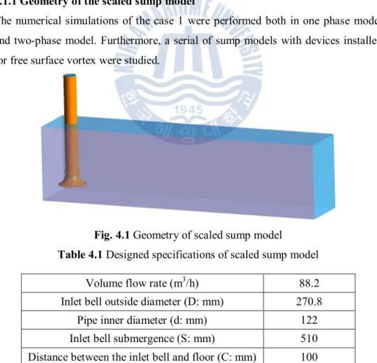
Fig. 4.1 Geometry of scaled sump model...33

Fig. 4.2 Schematic diagram of sump with anti free surface vortex devices...34

Fig. 4.3 Overall 3D drawing of the sump model...35

Fig. 4.4 2D drawing of the sump sketch...36

Fig. 4.5 Shape of the mixed flow pump...37

Fig. 4.6 Sump model with the submerged AVD...38

Fig. 4.7 Submerged AVD dimensions...39

Fig. 4.8 Overall mesh generation for scaled sump models...40

Fig. 4.9 Overall sump fluid domain mesh for the pump sump model...41

Fig. 4.10 Grid details of the pump sump model...41

Fig. 4.11 Boundaries of the scaled sump...43

Fig. 4.12 Experimental setup for the scaled sump model...46

Fig. 5.1 Streamline pattern of free surface...47

Fig. 5.2 Vortex core region of the sump model...48

Fig. 5.3 Velocity vectors on different sections...48

Fig. 5.4 Velocity vectors of PIV results...51

Fig. 5.6 Velocity vectors on free surface of different cases...53

Fig. 5.7 Tangential velocity profile of different models...55

Fig. 5.8 Performance curve of the mixed flow pump with the sump ...57

Fig. 5.9 Streamline pattern around the intake structure...58

Fig. 5.10 Vortex core region of the pump sump model...59

Fig. 5.11 Vorticity distribution in the flow direction...60

Fig. 5.12 Vorticity distribution in channel width direction...61

Fig. 5.13 Cavitation region of the mixed flow pump...62

Fig. 5.14 Cavitation performance curves of the mixed flow pump...63

Study of Flow Field in Rectangular Sump Models and

Performance Analysis of a Mixed Flow Pump

Yuxin ZHAO

Department of Mechanical Engineering

Graduate School of Korea Maritime and Ocean University

Abstract

It is an accepted fact that quite a number of problems faced in a pumping station are related to the design of sump or intake rather than pump design. Head-capacity curves provided by the pump manufacturer are obtained on the condition of no vortices flowing into the pump intake. The efficiency and performance of pumping stations depend not only on the performance of the selected pumps but also on the proper design of the intake sumps. A faulty design of pump sump can lead to the occurrence of swirl and vortices, which reduce the pump performance and induce vibration and additional noise. Therefore, sump model test is necessary to check the flow condition around intake structure. Numerical simulation is a good facility for reducing the time and cost involved throughout the design process. In this study, the commercial software ANSYS CFX-13.0 has been used for the CFD analysis of the sump models.

In a scaled sump model for air entrainment simulation, numerical analysis of single phase and two-phase with SST turbulence model was carried out to predict vortex (both free surface vortex and submerged vortex) occurrence and location. The effectiveness of curtain walls and square bars to eliminate the free surface vortex is evaluated. Meanwhile, the experiment including PIV system was performed in KMOU to investigate the flow conditions around pump intake structure.

In a full size sump model, overall numerical analysis for the sump model with a mixed flow pump installed was carried out. Hydraulic performances of the mixed flow pump for head rise, shaft power, pump efficiencies versus flow rate changed

from 50% to 140% of the design flow rate were studied by the performance curves. A trident shaped anti vortex device (AVD) composed of three wall fillets and one center splitter was installed under the pump intake. The effectiveness of the AVD for the suppression of submerged vortex was evaluated. In addition, numerical simulation of cavitation phenomenon in the mixed flow pump has been performed by calculating the full cavitation model with k-ε turbulence model.

According to the results, details of the location, size and strength of vortices were predicted in the numerical simulation. For the scaled sump model, although there is a little difference between the single phase and two-phase simulation, all the results predict the free surface vortex and submerged vortex formation and location. The CFD simulations of flow condition show good agreement with the PIV results. The effectiveness of curtain walls installed to inhibit the free surface vortex is confirmed in the CFD results; while the square bars installed in the channel failed to suppress the free surface vortex. For the mixed flow pump with sump, the best efficiency point (BEP) is at the design flow rate with the corresponding efficiency of 89.6%. The effectiveness of AVDs installed for the submerged vortex is confirmed by comparisons of the sump model with and without AVD results.

Cavitation phenomenon analysis shows the pump operating at the BEP condition has a considerable extent over the requirement of cavitation performance. With numerical simulation, the inception of cavitation in the blade passage is observed on the suction surface where the leading edges meet the tips, and then as the inlet total pressure decrease, the cavitation zone is spread out over the suction surface as well as the leading edge of the impeller blade.

Nomenclature

B: Distance from the back wall to the pump inlet bell centerline [m] C: Distance between the inlet bell and floor [m]

D: Inlet bell design outside diameter [m]

Fr: Froude number (=Vb/(g*D)0.5) [-]

g: Acceleration due to gravity [m/s2_]

ht: Total head [m]

n: Number of revolution per min [-]

Pflow: Flow power [W]

Pshaft: Shaft power [W]

Pν: Vapor pressure [Pa]

Q: Volume flow rate [m3_/s]

Q0: Design volume flow rate [m3/s]

Re: Reynolds number (=Vb*D/ν) [-]

S: Minimum submergence depth [m]

Vb: Velocity at bell mouth [m/s]

α： Angle of floor slope [°]

η: Pump efficiency [%]

θ: Swirl angle [°]

λ: The scale ratio of model dimensions to prototype [-]

μ: Viscosity [Pas]

ν: Kinematic viscosity [m2_/s]

ρ： Specific water density [kg/m3_]

σ: Surface tension [N/m]

Abbreviations

AVD Anti vortex device

BEP Best efficiency point

CFD Computational fluid Dynamics NPSH Net positive suction head

NPSHR Required net positive suction head

PIV Particle Image Velocimetry

RANS Reynolds Averaged Navier- Stokes RPM Number of revolutions per minute SST Shear Stress Transport

Chapter 1 Introduction

1.1 Background

It is an accepted fact that quite a number of problems faced in a pumping station are related to the design of sump or intake rather than pump design. As an important part of the pumping station, sump is designed to provide uniform, swirl and entrained air free flow to the pump intake. Undesirable flow conditions (entrained air, non-uniform flow distribution, vortices, etc.) can reduce the pump efficiency, induce vibration, noise and cavitation, even lead to excessive bearing loads of impeller and structure damage. Due to quite complex nature of the flow, although the flow conditions causing pump problems are well established, there are no specific solutions to eliminate them. There are some design guidelines for the specific geometrical and hydraulic constraints of the pump sump, for any project, the model study is the only tool for solving potential problems in new designs and rectifying problems observed in existing installations. However, the scaled model tests are expensive and time-consuming, so alternative Computational Fluid Dynamics (CFD) methods for evaluating sump performance have been developed. With rapid progress in CFD, numerical simulation is regarded as an effective tool in solving fluid problems in pump sumps.

1.2 Previous study

Various researches show the flow conditions around the sump intake structure are quite complicated. Shyam et al. [1] used the commercial code CFX to carry out two-phase flow simulation to capture air entrainment. The air entrainments and its location were well captured and numerical results were in accordance with the experimental investigation. Matsui J[2] and Okamura T[3] et al. conducted a serial research of the benchmark according to the Turbomachinery Society of Japan (TSJ) standard, including various commercial codes comparison performed in the flow simulation and comparison analysis between the numerical and experimental results.

The purpose of the benchmark is to determine the accuracy and reliability of the CFD codes used in universities and the industrial field. It is also intended to identify and investigate the formation of air-entrained and submerged vortices near the pump. Tanweer et al.[4] have performed a numerical analysis of a multiple intake pump sump to confirm that the geometry of sump affects the flow within sump greatly. Rajendran et al.[5] have made a numerical analysis for the flow characteristics of a sump model with pump intake and good agreements were achieved by comparing the numerical results with the experiments. Iwano et al.[6] have introduced a numerical method for the submerged vortex by analyzing the flow in the pump sump with and without baffle plates. Lee et al.[7] have conducted the CFD analysis of a multi-intake pump sump model to check the flow uniformity by predicting the location, number and vorticity of the vortex. For the CFD application in mixed flow pump design and performance analysis, Oh H W [8] conducted a mixed flow pump design optimization with specific parameters and then compared the numerical results with the experiments. The procedure presented can be used as a practical design and analysis guide for the general turbomachinery. Kim et al.[9] carried out a mixed flow pump performance analysis with numerical simulation and improved the hydraulic efficiency by the modification of the geometry.

As an undesirable phenomenon caused by the adverse flow condition, cavitation is the process of the formation of vapor bubbles within a liquid where flow dynamics cause the low pressure. With the rapid formation, growth and collapse of the bubbles, cavitation manifests in the form of pump performance decrease, vibration, additional noise increase and even the equipment damage. The cavitation phenomenon has been studied by various investigators. Van et al.[10] have investigated the cavitation inception behavior of a mixed-flow pump impellers model and the calculated results matched well with the experiments. Okamura et al.[11] have evaluated two numerical cavitation prediction methods used in the pump industry manufacturers, and attempts were made to improve the cavitation

development liquid/vapor interface tracking method to predict the cavitation characteristics with a centrifugal pump impeller model.

Moreover, there are a number of correlated studies [13]~[17].

1.3 Methodology of study

This study will investigate the flow phenomena of two sump models.

A scaled sump model is adopted to carry out numerical simulation and PIV experiment. The flow conditions are predicted and the effectiveness of devices for free surface vortex is evaluated; by using numerical code, a single intake sump model with a mixed flow pump installed is modeled and the hydraulic performance characteristics for the head rise, shaft power and pump efficiencies versus flow rate are studied. In addition, flow phenomena (vortices, cavitation, etc.) are analyzed and the effectiveness of an anti-vortex device (AVD) for the submerged vortex is evaluated.

Chapter 2 Basic theory of sump model

Specific hydraulic phenomena have been confirmed that they can lead to certain common operational problems. The common of the main problems are summarized as follows:

a. Free surface vortices; b. Submerged vortices;

c. Swirl of flow entering the pump;

d. Non-uniform distribution of velocity at the pump impeller; e. Entrained air or gas bubbles.

These problems encountered in the pump sump will affect the pump performance and significantly increase the operational and maintenance costs. In order to identify sources of particular problems and find practical solution for it, the usual approach is to conduct the laboratory experiments on a scaled physical model. Typical design objectives are to ensure that a pump station is designed according to best practice and conforms to the requirements set out in the American National Standard for Pump Intake Design[18]. These standards restrict the degree to which the above-mentioned undesirable flow patterns may be present. The negative impact of each of these hydraulic conditions varies with pump specific speed and size. Application of the standard to design a sump does not generate a problem free sump but provides a basis for the initial design.

As there are no specific guidelines or criteria for design of trouble free intakes, the most common solution to potential problems in new design and rectification of problems observed in existing designs is to construct a scaled model in a laboratory, observe and investigate the flow characteristics and propose modifications to the intake geometry. There are additional devices in the form of floor splitters or cones, back wall splitters, fillets, surface beams, guide vanes etc, aimed at controlling the vortex and swirl formation. Considerable prior experience and ingenuity are

required to solve the problems by this method and the cost and time required are also significant.

The intake structure refers to the channel leading from the water source which may be a river or reservoir and all installations downstream including the pump column or the intake pipe (the suction tube portion of a vertical intake), the approach channel (upstream of pump bay) and the pump bay (bounded by the floor, the back wall, side walls dividers walls separating adjacent pump column). Usually the upstream end of the pump column has an inlet attachment called the suction bell. The function of the intake is to supply an evenly distributed flow of water to the pump suction bell.

Several types of pump intake basins are available and ANSI/HI 9.8 provides design requirements for each. Intake structures can be categorized as being clear liquids or solids-bearing liquids. For clear liquids, intakes are further classified into rectangular, formed, circular and trench types, as well as suction tanks and cans. For solid-bearing liquids, trench type and rectangular wet wells are usually considered.

In this paper, only rectangular intake structure for clear liquid is studied.

2.1 Pump intake design

For pumps to achieve their optimum hydraulic performance across all operating conditions, the flow at the impeller must meet specific hydraulic conditions. The ideal flow entering the pump inlet should be of a uniform velocity distribution without rotation and stable over time. When designing a sump to achieve favorable inflow to the pump or suction pipe bell, various sump dimensions relative to the size of the bell are required. Using these standards of the distances to reduce the probability of the occurence of strong submerged vortices and free-surface vortices.

2.1.1 Inlet bell diameter design

The geometry is generally defined in terms of the pump inlet diameter as shown in Table 2.1 and Fig. 2.1. The bell diameter can be estimated based on an inlet pipe velocity.

Table 2.1 Acceptable velocity ranges for inlet bell diameter(ANSI/HI 9.8)

Flow Rate Q，l/s

Recommended Inlet Bell Design Velocity，m/s Acceptable Velocity Range, m/s Q＜315 V=1.7 0.6≤V≤2.7 315 ≤Q＜1260 V=1.7 0.9≤V≤2.4 Q ≥1260 V=1.7 1.2≤V≤2.1

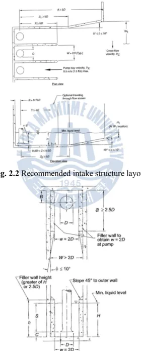
2.1.2 Recommended dimensions for a rectangular sump

As the selected bell diameter has been determined, the proportions of the inlet structure can be estimated from Fig. 2.2 and Fig. 2.3. Table 2.2 shows the recommended dimensions for a rectangular sump.

Fig. 2.2 Recommended intake structure layout

Table 2.2 Recommended dimensions for a rectangular sump Dimension

Variable Description Recommended value

A Distance from the pump inlet bell

centerline to the entrance A=5D minimum a Length of constricted bay section near

the pump inlet 2.5D minimum B Distance from the back wall to the

pump inlet bell centerline 0.75D C Distance between the inlet bell and _floor 0.3D~0.5D

D Inlet bell outside diameter refer to section 2.1.1

H Minimum liquid depth H=S+C

h Minimum height of constricted bay

section near the pump inlet bell h>H or 2.5D S Minimum pump inlet bell submergence S=D(1.0+2.3Fr)

W Pump inlet bay entrance width 2D minimum

w Constricted bay width near the pump _{inlet bell} w=2D

X Pump inlet bay length 5D minimum

Y centerline to the through-flow traveling Distance from pump inlet bell screen

4D minimum

Z1 Distance from sump inlet bell _{centerline to diverging walls} 5D minimum

Z2 Distance from inlet bell centerline to _{sloping floor} 5D minimum

α Angle of floor slope -10°~ +10°

β Angle of wall convergence 0°~ +10°

FD=Vb/(g*D)0.5 (2.1)

where

FD : Froude number (dimensionless)

Vb: velocity at suction inlet=Flow/Area, based on D

D: Outside diameter of bell or pipe inlet g: gravitational acceleration

There is the design sequence summary for rectangular intake structures:

· Consider the flow patterns and boundary geometry of the body of liquid from which the pump station is to receive flow. Compare with the approach flow condition and determine if a hydraulic physical model study is required.

· Determine the number and size of pumps required to satisfy the range of operating conditions likely to be encountered.

· Identify pump inlet bell diameter. Refer to the section 2.1.1.

· Determine the bell-floor clearance, 0.5D is a good preliminary design value. · Determine the required bell submergence, using the equation 2.1.

· Determine the minimum allowable liquid depth in the intake structure from the sum of the floor clearance and the required bell submergence.

· Check bottom elevation near the entrance to the structure and determine if it is necessary to slope the floor upstream of the bay entrance. If the resulting depth at the entrance to the intake structure is shallow, then check to ensure that gravity-driven flow is not restricted by the entrance condition.

· Check the pump bay velocity for the maximum single-pump flow and minimum liquid depth with the bay width set to 2D. If bay velocity exceeds 0.5 m/s, then increase the bay width to reduce the maximum velocity below 0.5 m/s .

· If it is necessary to increase the pump bay width to greater than 2D, then decrease bay width in the vicinity of the pumps according to Fig. 2.3.

· Compare cross-flow velocity (at maximum system flow) to average pump bay velocity. If cross-flow value exceeds 50% of the bay velocity, a physical hydraulic model study is necessary.

· Determine the length of the structure and dividing walls, giving consideration to minimum allowable distances to a sloping floor, screening equipment, and length of dividing walls ,if dual flow traveling screens or drum screens are to be used, a physical hydraulic model study is required. · If the final selected pump bell diameter and inlet velocity is within the

range given in section 2.1.1, then the sump dimensions (developed based on the inlet bell design diameter) need not be changed and will comply with these standards.

2.2 Model test

The approach flow pattern in a pump intake facility is difficult to predict by traditional mathematics or empirical formulae. For large structures or those that differ significantly from proven designs, a model study is the only means to ensure success. A model study is used to identify adverse hydraulic conditions and derive remedial measures for approach flow patterns generated by structures upstream of the pump impeller. Current model studies are not intended to investigate flow patterns induced by the pump itself or the flow patterns within the pump. The objective of a model study is to ensure that the pump intake structure generates favorable flow conditions at the inlet to the pump. Evaluation for the requirement of model test if:

a: Sump or piping geometry that deviates from this design standard.

b: Non-uniform or non-symmetric approach flow to the pump sump exist.

c: The pumps have flows greater than 2520 l/s per pump or the total station flow with all pumps running would be greater than 6310 l/s.

Adverse hydraulic conditions that can affect pump performance include: free and submerged vortices, swirl approaching the pump impeller, flow separation at the pump bell, and a non-uniform axial velocity distribution at the suction.

The purpose of model test is to examine these adverse hydraulic conditions and to investigate measure against them.

2.2.1 The scale effects

One possible difficulty in scale modeling is that it is impossible to reduce all pertinent forces by the same factor. With Froude-scale models, the inertial and gravitational forces are reduced similarly, but the viscous and surface tension forces cannot be simultaneously reduced. The extra influence of these forces is known as a “scale effect”. A number of investigations have indicated that the scale effects for the model are avoided if the Reynolds number, based on the inlet flow and submergence or intake diameter, exceeds approximately 3x 104 _{, and the Weber}

number exceeds 150 [19].

In most engineering applications involving closed-conduit and open-channel flow, the Reynolds number limits are far exceeded and the flows are fully turbulent. In a sump model, Froude number (Fr) and Reynolds number (Re) are the most important non-dimensional parameters. Some reduction in Re should be introduced to the sump model. However, flow patterns are generally very similar at high Re.

No specific geometric scale rate is recommended, but reasonable large geometric scale to minimize viscous and surface tension scale effects and reproduce the flow pattern.

Re= uD/ν (2.2)

We= u2ρD/σ (2.3)

where

u: average axial velocity (m/s)

ρ: liquid density (kg/m3₎

σ: surface tension of liquid/air interface

According to the ANSI/HI 9.8, the viscous scale effects on vortex may be negligible if the resulting dimensionless numbers must meet these values : Re＞6×104 and We＞240

To allow practical visual observations of flow patterns, accurate measurements of swirl and velocity distribution, and sufficient dimensional control, the model scale shall yield a bay width of at least 300mm, a minimum liquid depth of at least 150mm, and a pump throat or suction diameter of at least 80mm.

2.2.2 Principle of similarity

In the similitude analysis, the geometric and flow similarity requires the model and the flow to be identical as the real model and flow. This is to ensure the result obtained from the model study is well presented in order to predict full scale behavior. Model involving a free surface are operated using Froude similarity since the flow process is controlled by gravity and inertial forces.

For similarity of the flow patterns, the Froude number shall be equal in model and prototype.

Fr = =

(2.4)

and as the scale ratio λ was selected in section 2.2.1, the following equation is obtained:

V = V × ( ) . _{= V × λ} . _{or Q = Q × ( )} . _{= Q × λ} . _(2.5)

where Fris the Froude number, λ is the scale ratio of model dimensions to prototype. The test of 1.5 times Froude scaled flow should be conducted to ascertain the potential scale affect on free surface vortices.

Models of closed conduit piping system leading to a pump suction are not operated based on Froude similitude. However, flow patterns are generally very similar at high Re. A minimum value of 1×105 _{for the Re at the pump suction is}

2.2.3 Preliminary model test

The initial design shall be tested first to identify any hydraulic problems.

1) Vortex Formation Mechanisms:

There are various investigations that provide insight into the fundamental processes leading to the development of vortices both in experiment and numerical simulation. Shin et al. [20] demonstrated that two basic mechanisms lead to inlet vortex formation. The first mechanism involves the development of an inlet vortex due to the amplification of ambient vorticity in the approach flow as vortex lines are convicted into the inlet. The second mechanism involves the development of a trailing vortex in the vicinity of the intake as a result of the variation in circulation along the inlet. For this second case, a vortex can develop in a flow that is irrotational upstream, and the vortex development therefore does not depend on the presence of ambient vorticity. Shin et al. investigation on kinematic parameters, indicate that the strength of an inlet-vortex or trailing vortex system increases with decreasing distance from the surface. However, for an inlet in an upstream irrotational flow, two counter rotating vortices can still trail from the rear of the inlet.

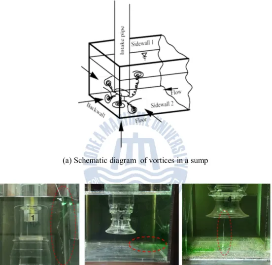
2) Classification of vortex type:

As illustrated in Fig. 2.4, vortices in the vicinity of pump intakes may be adjacent to the channel bottom or a channel wall (i.e. submerged vortices) or they may appear adjacent to the free surface (i.e. free surface vortex).

(a) Schematic diagram of vortices in a sump

(b) Experimental results of different vortex

For the model visual observation, dye was injected around the intake structure near the surface and submergence as Fig. 2.4 (b) shows. And the model test results of vortex was classified as Fig. 2.5.

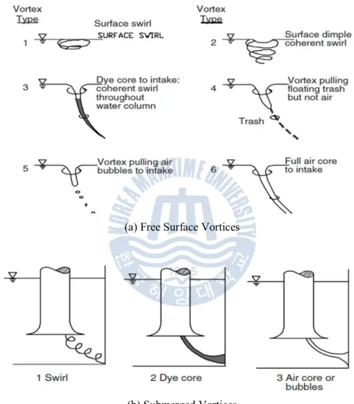
(a) Free Surface Vortices

(b) Submerged Vortices

Fig. 2.5 Vortex classifications

There are a number of researches focused on the numerical theory to detect the inception of a visible vortex. As the diameters of vortices are usually much smaller compared with the computing grid size, to compensate for the lack of vortex resolution in numerical simulation, a stretching vortex model is applied to the local

flow field around semi-analytically identified vortex positions [21][22]. The brief explanations are as follows:

a) Free surface vortex

The criteria expressed by equation 2.6 and 2.7 is applied to determine the visible inception of a free surface vortex,

≫ 1 (2.6)

= > 1 (2.7)

where _P is the pressure drop at the vortex core and _Ph is the static head at the

vortex element, and _f is the drag force acting at a unit length of water surface vortex dimple, based on Stokes approximation and caused by the down flow. Further, _f is the force acting on the bubble in the direction from the high pressure region to the low pressure region like buoyancy.

b) Submerged vortex

Equation 2.8 is applied to determine the visible inception of a submerged vortex.

∆

∞ = ∞

∞ > 1 (2.8)

where is the static pressure at the vortex core, ∞ is the atmospheric pressure and _{is the critical cavitation inception pressure and nearly equal to the} saturated vapor pressure.

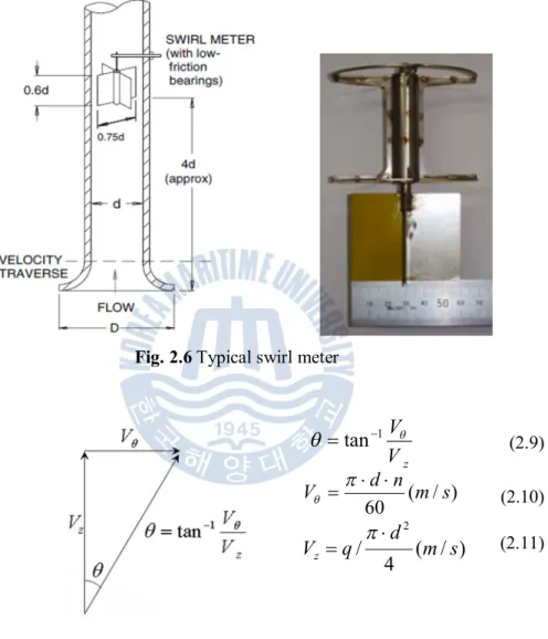
3) Swirl angle：

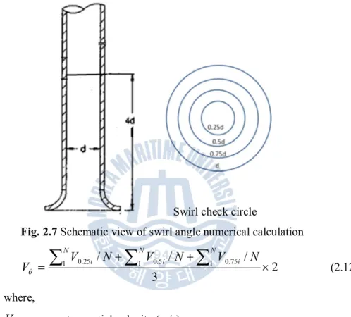
Swirl angle predicts the intensity of flow rotation. Fig. 2.6 shows experiment calculation method with swirl meter, and attempts of the CFD calculation method were conducted as Fig. 2.7. A four blade zero-pitch swirl meter, which is supported by a low friction bearing, will be installed at about four suction pipe diameter (d) downstream from the pump suction to measure swirl angle of pump approaching flow. For the swirl meter, the tip to tip blade diameter is 0.75d and the length in flow direction is 0.6 and one of the four blade is painted yellow as a reference to

count revolutions. As flow swirl is usually unsteady, the observation time of swirl meter reading should be a continuous period of time.

Fig. 2.6 Typical swirl meter

(2.9) (2.10) (2.11)

Where,

V

d

q

V

V

q

₌

_tan

p

)

/

(

4

/

s

m

d

q

V

×

=

p

For the swirl angle calculating method with CFD, the key point is to obtain the average tangential velocity, so the swirl check circles were created as illustrated in Fig. 2.7. The swirl check circle is located at the section of 4d height with diameter of 0.25d, 0.5d and 0.75d, respectively.

Swirl check circle

Fig. 2.7 Schematic view of swirl angle numerical calculation

2 3 / / / 1 0.75 1 0.5 1 0.25 + + _´ =

å

å

å

V

V

N

4) Velocity:

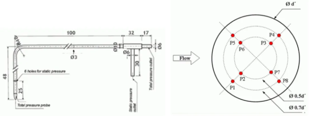
Velocity measurement at bell throat by Pitot tube was implemented by ANSI/HI method. Typical Pitot tube configuration is shown in Fig. 2.8. Eight measuring points are defined as Fig. 2.9. Time averaged velocity at eight points was obtained and these eight data were again averaged to give throat sectional spatial velocity

Fig. 2.8 Example of Pitot tube Fig. 2.9 Measuring points at bell throat 2.2.4 Test criteria

There is the criteria for satisfactory performance of the sump model test and summarized in Table 2.3.

1) Free surface and submerged vortices:

Free surface vortices entering the pump must be less severe than vortices with coherent core; Dye core vortices may be acceptable only if they occur less than 10% of the time or only for infrequent pump operating conditions.

Submerged vortex which starts from the sump walls induce vibration and noise problems. Dye core submerged vortices extending into the pump bell mouth is not allowed.

2) Swirl angles:

Swirl angle is used to check the flow rotation in the suction pipe. The calculation

method is referred to section 2.2.3.

Short-term maximum and long-term average values must be less than 5 degrees. Maximum short-term swirl angles up to 7 degrees may be acceptable only if they occur less than 10% of the time or only for infrequent pump operating conditions.

3)Velocity:

Each point time-averaged velocity shall not be larger than 10% of sectional average velocity.

Standard deviation of time-varying velocity at each point was obtained, and its value shall not be larger than 10% of the time-averaged velocity at each point. 1) Time-averaged Variation[%] =

-

´

100

V

V

V

V

-å

Variation[%] = (Standard deviation /

X

X

Table 2.3 Permission criteria of ANSI/HI

Vortex occurence Swirl angle

Free surface vortex Submerged vortex

Observation

time Above 10 minutes Above 10 minutes

Above 10 minutes Permission criteria Dye-core Vortex(F3), below 1/10 total time Dye-core Vortex(S2), below 1/10 total time Below 5°,Conditional intermittent below 7°

2.2.5 Remedial measures for problem intakes

Usually in the preliminary test, the worst flow condition is simulated. And based on the results, remedial measures for problem intakes are discussed in this part.

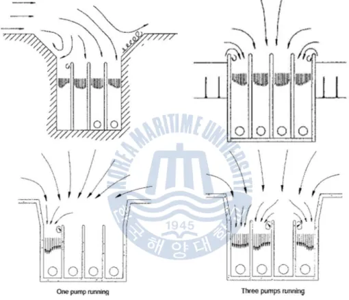
1) Overall approach flow patterns:

The characteristics of flow approaching an intake structure is one of the foremost considerations for the designer. It is difficult to predict the effects of a given set of flow conditions upstream from an intake structure. Fig. 2.10 depicts several typical approach flow patterns of pump sump with different operating conditions.

Fig. 2.10 Examples of approach flow patterns

Generally speaking, for the intake problems, especially for the multiple pumps sump, there are the main measures: using dividing walls placed between the pumps as a partitioned structure; trash racks with elongated bars, guide piers or a number of structural columns at the bay entrance can provide some assistance in controlling cross-flow; baffles, flow distributors and screen mesh, etc are applied to improve the flow distribution.

2) Problems around pump intake: a) Free surface vortices:

There are a number of factors that have an effect on the formation of surface vortices. To achieve a higher degree of certainty that objectionable surface vortices do not form, modifications can be made to intake structure to allow operation at practical depths of submergence and the minimum submergence is referred in Table 2.2, the use of suction umbrellas, vertical curtain walls and horizontal gratings.

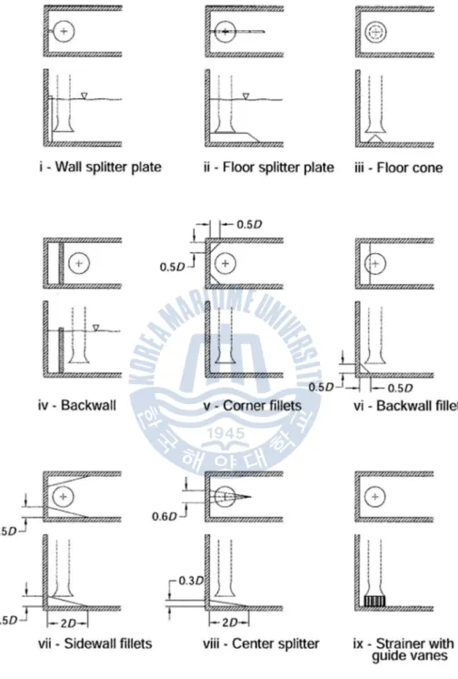
b) Submerged vortices:

In the vicinity of intake bell, there are the most complicated flow patterns and flow makes the most changes in direction, while maintaining a constant acceleration into the pump bell to prevent local flow separation, turbulence and vortex formation. Fig. 2.11 represents a sample of various devices to inhibit the different submerged vortex.

c) Preswirl:

The approach flow distributions determine whether flow preswirl exists and a sufficiently laterally skewed approach flow cause rotating around the intake bell. The most effective way of reducing preswirl is to establish a relatively uniform approach flow within each pump bay by using the baffling schemes, controlling cross-flow and expanding concentrated flow discussed in the above part.

To prevent non-uniform velocity distribution, swirls and vortices , necessary modifications are conducted, such as fore bay length, baffle wall, distributors, curtain wall, mesh screen, guide vane, floor splitter, wall fillet, etc. As the above measures applied, modification test will be conducted to check all the flow conditions and compare with the preliminary results.

Chapter 3 Methodology

CFD (Computational fluid dynamics) is the technique, which can design cycles to better performance and reduce costs and time. In CFD, we solve the governing equations of given physics (may be differential form or integral form) using some numerical techniques like Finite Difference Method (FDM), Finite Element Method (FEM) or Finite Volume Method (FVM). Although CFD plays a great part in the design of turbomachinery, CFD is not a replacement for experimental or analytical approach. In this study, the numerical analysis was performed by the commercial code ANSYS CFX 13.0. All aspects of the CFD study including modelling , meshing, solving and post-processing of the results.

3.1 Numerical modeling

ANSYS CFX solves the unsteady Navier-Stokes equations in their conservation form. The instantaneous equation of mass (continuity) in the stationary frame is expressed as equation:

ρ

δ + ∇ ∙ (ρU) = 0 (3.1)

And the instantaneous equation for momentum is expressed as shown in equation:

ρ

δ + ∇ ∙ (ρU⨂U) = −∇p + ∇ ∙ τ + S (3.2)

Where τ is the stress tensor ( including both normal and shear components of the stress).

These instantaneous equations are averaged for turbulent flows leading to additional terms that need to be solved. While the Navier-Stokes equations describe both laminar and turbulent flows without addition terms, realistic flows involve length scales much smaller than the smallest finite volume mesh. A Direct Numerical Simulation of these flows would require significantly more computing power than what is available now or in the future.

Therefore, much research has been done to predict the effects of turbulence by using turbulence models. These models account for the effects of turbulence without the use of a very fine mesh or direct numerical simulation.

These turbulence models modify the transport equations by adding averaged and fluctuating components. The transport equations are changed to equations (3.3) and (3.4):

ρ

δ + ∇ ∙ (ρU) = 0 (3.3)

ρ

+ ∇ ∙ {ρ U ⨂U} = −∇p + ∇ ∙ τ − ρu⨂u + S (3.4)

The mass equation is not changed but the momentum equation contains extra terms which are the Reynolds stresses, ρ _{u⨂u and the Reynolds flux, ρ u ϕ . These} Reynolds stresses need to be modeled by additional equations to obtain closure. Obtaining closure implies that there are a sufficient number of equations to solve for all the unknowns including the Reynolds stresses and Reynolds fluxes.

Various turbulence models provide various ways to obtain closure. In this investigation, Shear Stress Transport (SST) model and k-ε model were utilized. The advantage of SST model is that combines the advantages of other turbulence models (the k-ε, Wilcox k-ω). The 3 turbulence models will be discussed briefly.

3.2 Turbulence models

Turbulence models are necessary because we cannot afford big enough computers to directly capture every scale of motion. There are three modelling frameworks: Direct Numerical Simulation (DNS); Reynolds-Averaged Navier-Stokes Equations(RANS); Large Eddy Simulation(LES).

As RANS method is applied in most production，several RANS turbulence models differ in their usage of wall functions, the number of additional variables solved for, and what these variables represent.

Two equation turbulence models:

Two-equation turbulence models are widely used in CFD as they give a good compromise between computational power needed and accuracy. The term ‘two equation’ refers to the fact that these models solve for the velocity and length scales using separate transport equations. The turbulence velocity scale is obtained by solving the transport equation. The turbulent length scale is estimated from two properties of the turbulence field, namely the turbulent kinetic energy and the dissipation rate. The dissipation rate of the kinetic energy is obtained from its transport equation. The most widely used are k-ε and k-ω two equation models. In the next section, the k-ε, Wilcox k-ω, BSL k-ω and SST models will be briefly discussed.

3.2.1 k-ε turbulence model

The k-epsilon model solves for two variables: k; the turbulent kinetic energy, and epsilon; the rate of dissipation of kinetic energy. Wall functions are used in this model, so the flow in the buffer region is not simulated. The k-epsilon model is very popular for industrial applications due to its good convergence rate and relatively low memory requirements. It does not very accurately compute flow fields that exhibit adverse pressure gradients, strong curvature to the flow, or jet flow. It does perform well for external flow problems around complex geometries.

The k-ε model introduces k (m2_/s2_{) as the turbulence kinetic energy and ε (m}2_/s3_{) as}

the turbulence eddy dissipation. The continuity equation remains the same:

ρ

+ ∇ ∙ (ρ U) = 0 (3.5)

The momentum equation changes, as shown by equation:

δρ

δ + ∇ ∙ (ρU⨂U) = −∇p

′_{+ ∇ ∙ μ}

∇U + (∇U) + S (3.6)

Where SM is the sum of body forces, μeff is the effective viscosity accounting for

turbulence and p’ is the modified pressure. The k-ε model uses the concept of eddy viscosity giving the equation for effective viscosity as shown by equation:

μt is the turbulence viscosity is linked to the turbulence kinetic energy and

dissipation by the equation:

μ _{= C}μρ _ε (3.8)

Where Cμ is a constant.

The values for k and ε come from the differential transport equations for the turbulence kinetic energy and the turbulence dissipation rate.

The turbulence kinetic energy equation is given as equation:

(ρ )

+ ∇ ∙ (ρUk) = ∇ ∙ μ + μ

σ ∇k + P + P − ρε (3.9)

The turbulence dissipation rate is given by equation:

(ρε) + ∇ ∙ (ρUε) = ∇ ∙ μ + μ σ_ε ∇ε + ε (Cε (P + Pε ) − Cε ρε) (3.10)

Where Cε1, Cε2, σk, σε are constants.

Pk is the turbulence production due to viscous forces and is modeled by the equation:

P = μ ∇U ∙ ∇U + ∇U − ∇ ∙ U 3μ ∇ ∙ U + ρk (3.11) If a buoyancy term is added to the previous equation if the full buoyancy model is used.

The buoyancy term Pkb is modeled as:

P = −_ρσμ_ρg ∙ ∇ρ (3.12)

3.2.2 Wilcox k-ω turbulence model

The k-omega model is similar to k-epsilon, instead however, it solves for omega — the specific rate of dissipation of kinetic energy. It also uses wall functions and therefore has comparable memory requirements. It has more difficulty converging and is quite sensitive to the initial guess at the solution. Hence, the k-epsilon model is often used first to find an initial condition for solving the omega model. The k-omega model is useful in many cases where the k-epsilon model is not accurate, such as internal flows, flows that exhibit strong curvature, separated flows, and jets.

This model has an advantage over the k-ε model, where it does not involve complex linear damping functions for near wall calculations at low Reynolds numbers. The k-ω model assumes that the turbulence viscosity is related to the turbulence kinetic energy, k, and the turbulent frequency, ω, by the equation:

μ _{= ρ ω} (3.13)

The transport equation for k is given by the equation:

(ρ )

+ ∇ ∙ (ρUk) = ∇ ∙ μ + μ

σ ∇k + P + P − β

′_{ρ k ω (3.14)}

The transport equation for ω is shown as equation:

(ρω) δ + ∇ ∙ (ρ U ω) = ∇ ∙ μ + μ μ_ω ∇ω + α ω P + Pω − β ρ ω (3.15)

The production rate of turbulence (Pk) is calculated as shown previously in the k-ε

section.

The recommended values for the constants in the above equations are: β′_{= 0.09,}

α_{= 5 9} , β_{= 0.075,} σ _{= 2,} σω= 2.

The Reynolds stress tensor, ρ _{u⨂u, is calculated by:}

−ρ u⨂u = μ ∇U + (∇U) − ∂ ρk + μ ∇ ∙ U (3.16)

3.2.3 Shear stress transport model

The disadvantage of the Wilcox model is the strong sensitivity to free-stream conditions. Therefore a blending of the k-ω model near the surface and the k-ε in the outer region was made by Menter [23] which resulted in the formulation of the BSL k-ω turbulence model. It consists of a transformation of the k-ε model to a k-ω formulation and subsequently adding the resulting equations. The Wilcox model is multiplied by a blending function F1 and the transformed k-ε by another function

1-F1. F1 is a function of wall distance (being the value of one near the surface and zero

outside the boundary layer). Outside the boundary and on the edge of the boundary layer, the standard k-ε model is used [24].

SST model is a combination of the k-epsilon in the free stream and the k-omega models near the walls. It does not use wall functions and tends to be most accurate when solving the flow near the wall. The SST model does not always converge to the solution quickly, so the k-epsilon or k-omega models are often solved first to give good initial conditions.

The k-ω based Shear Stress Transport (SST) model of Menter was applied for turbulence treatment. The transport equations for the SST model are expressed below where the turbulent kinetic energy ‘k’ and turbulent frequency or dissipation per unit turbulent kinetic energy ' ' are computed by using the following relations:

For Turbulence Kinetic Energy,

k k P uk t k T k k - +Ñ + Ñ = Ñ + ¶ ¶ ) .[( ) .(

_b

_w

_n

_s

_n

where Pk is the production limiter. For Specific Dissipation Rate,

w

w

s

w

n

s

n

bw

a

w

w

The first blending function F1 is calculated from

ïþ

ï

ý

ü

ïî

ï

í

ì

ïþ

ï

ý

ü

ïî

ï

í

ì

ú

ú

û

ù

ê

ê

ë

é

÷÷

ø

ö

çç

è

æ

=

4

500

;

max

min

tanh

y

CD

k

y

y

k

F

rs

w

n

w

b

y is the distance to the nearest wall and v is the kinematic viscosity.

÷

ø

ö

ç

è

æ

_Ñ

_Ñ

=

.

,

10

1

2

max

w

w

rs

k

CD

And, Kinematic eddy viscosity,

)

,

max(

SF

k

_a

_w

a

n

=

where, F2 is a blending function which restricts the limiter to the wall boundary and S is the invariant measure of the strain rate.

ú

ú

û

ù

ê

ê

ë

é

ïþ

ï

ý

ü

ïî

ï

í

ì

÷÷

ø

ö

çç

è

æ

=

500

;

2

max

tanh

w

n

w

b

y

y

k

F

3.3 Brief introduction of simulation process

All aspects of CFD study including modelling , meshing, solving and post-processing of the results are briefly introduced in this chapter.

3.3.1 Pre-processing technique

The speed and accuracy of simulation results depending fundamentally on meshing and the ability to prepare model geometry correctly.

The steps in pre-processing are explained as follows: 1) Domain Definitions

The domain definition depends mainly on the physics involved in the problem and objective of the problem.

a) Geometry creation or geometry import b) Geometry cleanup

i) Removing the parts not necessary for simulation under consideration ii) Closing the gaps in the geometry

iii) Removing small surfaces, curves to make meshing process simple 2)Grid generation

To solve the governing equations, the numerical methods like Finite Difference, Finite Volume or Finite Element Method to divide the domain into small parts and solve the equations on one part at a time are applied.

3) Labeling (Putting Tags)

Applying boundary conditions in pre-processing tool is the process of putting appropriate tags (labels) on specific boundaries. There are typically two types of boundary conditions:

a) Surface boundary conditions: inlet, outlet, wall etc.

b)Domain(regions) boundary conditions: to specify the solid region or fluid region.

The data provided on boundaries (e.g. velocity at inlet, pressure at outlet etc.) is going to be used during solution of the governing equations.

3.3.2 Solving the simulation

Once the models have the various variables and boundary conditions specified, the following step is to solve for the solutions using a solver. This study used the CFX-Solver 13.0 software as the solver.

There are several techniques that can be used to solve the governing equations that were described earlier. CFX uses the Finite Volume Method (FVM) approach to solve the required equations.

3.3.3 Post processing

The post processing proceed after the required simulation is completed. Post Processing refers to processing the result of the simulation by a number of ways:

Generating a visual representation of various flow variables over the geometry;

Generating animations of flow vectors; Analyzing flow variable distributions; Processing of results for output onto a chart.

The ANSYS software provides CFX-Post as a Post processor function.

These steps combined with the specific model case will be further discussed in the next chapter.

Chapter 4 Description of Model Cases

This chapter gives methodology details of both cases: a scaled rectangular sump model and a full size sump model with a mixed flow pump installed. Meanwhile, the arrangement of PIV measurements is introduced.

4.1 Creating the geometry

The three dimensional models of the geometry for the sump fluid domain were made using the commercial code Unigraphics NX 6.0 according to the available design.

4.1.1 Geometry of the scaled sump model

The numerical simulations of the case 1 were performed both in one phase model and two-phase model. Furthermore, a serial of sump models with devices installed for free surface vortex were studied.

Fig. 4.1 Geometry of scaled sump model

Table 4.1 Designed specifications of scaled sump model

Volume flow rate (m3_{/h) 88.2}

Inlet bell outside diameter (D: mm) 270.8 Pipe inner diameter (d: mm) 122 Inlet bell submergence (S: mm) 510 Distance between the inlet bell and floor (C: mm) 100

Fig. 4.1 shows the shape of sump model. The width of intake channel is 500mm and the center of suction bell is located at 201mm, 250mm and 100mm from rear wall, side wall and bottom, respectively. The model (scale ratio 1:7.2 to prototype) was applying the Froude Number similarity principle and all the dimensions are confirmed to chapter 2.

e.g. S=D(1.0+2.3Fr) according to ANSI/HI; While Fr=Vb/(g*D)0.5

Solving, we got recommend minimum S=434mm ＜510mm.

As illustrated in the Schematic diagram of Fig. 4.2 and Table 4.2, the location and dimensions of anti free surface vortex device (curtain wall or square bar) are confirmed.

(a) Sump model with curtain wall

(b) Sump model with square bar

Table 4.2 Parameters of anti free surface vortex devices Case Distance to sump back wall (mm) Submergence of the bottom (mm) Dimensions below water surface (mm) Curtain wall 1 760 100 100×60×500 Curtain wall 2 760 200 200×60×500 Curtain wall 3 760 300 300×60×500 Square bar 1 760 200 100×50×500 Square bar 2 760 300 100×50×500

4.1.2 Geometry of the full size pump sump model 1) Model of the sump layout:

Fig. 4.3 shows the 3D overall sump model with the mixed flow pump installed.

As illustrated in Fig. 4.4 (a), the total flow direction length of the model is 30m, with a long channel of 2.6m in width, 18m in length and a baffle about 8.6m distance from the intake bell center. The width of the intake channel is 4m, and the center of the intake bell is located at 1.8m, 2m and 0.7m from rear wall, side wall and bottom, respectively. All the dimensions referred the recommended values of Chapter 2.

(a) Top view

(b) Side view

Fig. 4.4 2D drawing of the sump sketch

2) Model of the mixed flow pump:

Generally, pump is a mechanic equipment which is required to lift liquid from low level to high level or to flow liquid from low pressure area to high pressure area. Principally, pump converts mechanic energy of motor into fluid flow energy. Pumps are commonly rated by power, flow rate and total head. The head can be simplified

atmospheric pressure. From an initial design point of view, engineers often use a quantity termed the specific speed to identify the most suitable pump type for a particular combination of flow rate and head.

The blade profile of the mixed flow pump is created in BladeGen. Fig. 4.5 shows the 3D geometry and meridional geometry of the mixed flow pump and Table 4.3 provides the design specifications of the mixed flow pump.

(a) 3D geometry

(b) Meridional geometry

Table 4.3 Design specifications of the mixed flow pump

Volume flow rate (m3/h) 21,700 Rotational speed (rpm) 423

Total head (m) 23

Number of impeller blade 5

Number of diffuser vane 9

Impeller inlet diameter (m) 1.096

3) Sump model with the submerged AVD:

Fig. 4.6 shows the sump model with AVD installed. The AVD is designed to suppress the submerged vortex that occurs near the side wall and bottom.

Fig. 4.7 Submerged AVD dimensions

The trident shaped AVD installed under the pump intake is made up of three wall fillets (800mm height) and one central splitter (200mm height). The design of this AVD referred to Appendix A of the standard ANSI/HI 9.8.

4.2 Mesh generation

Mesh generation refers to the creation of a numerical domain over a certain geometry in which the computer can use to solve the required equations. After the completion of the geometry, a number of computer based software may be used to generate the numerical domain. In this study, ICEM CFD was used to generate the mesh of the sump fluid domain, while for the mixed flow pump grid generation, TurboGrid is used along with BladeGen.

ICEM CFD allows for the generation of several types of meshes including tetrahedral, hexahedral or even hybrid meshes. Tetrahedral meshes are generally less time consuming to build whereas hexahedral meshes provide more accurate results that the mesh quality is high.

In addition to this, ICEM CFD allows for the generation of structured or unstructured meshes. Structured meshes have cells that are regular in shape and each grid point is uniquely identified by indices and coordinates. Unstructured

meshes contain cells that are not necessarily regular in shape and have grid points in no particular ordering. The main advantage of unstructured meshes is the flexibility it provides in the generation of a computational grid in complex geometries.

The computational grid of all the geometries in this investigation was made of unstructured hexahedral volumes to ensure accurate results.

The flow domain was divided into a number of smaller regions for two reasons. Firstly, it improved mesh quality, and secondly it enabled named selections to be created. The mesh quality was noticeably improved by separating the flow domain in regions free from complex geometrical shapes. This is because a hexahedral mesh was easier to be applied for uniform volumes. Named selections were utilized to specify boundary conditions and to facilitate results viewing. These domains were meshed separately and imported to CFX-Pre forming one computational domain.

(a) Overall mesh generation for single phase model

As the overall mesh shows, the scaled sump model is divided into several parts to employ hexa-hedral mesh. The total nodes for the single phase model is about 1.65 millions and for the two-phase model is about 2.28 millions.

Fig. 4.9 Overall sump fluid domain mesh for the pump sump model

a) Tetrahedral mesh of Bell mouth b) Hexahedral mesh of the mixed flow pump

Fig. 4.10 Grid details of the pump sump model

Fig. 4.9 shows the overall mesh of the sump domain, as the complex fluid domain was divided into 5 parts, the girds were generated according to the geometry, separately. The grid details of bell mouth and the mixed flow pump are shown in Fig. 4.10.

Table 4.4 Mesh information for the pump sump model

Number of nodes Mesh type

Impeller domain 800,000 Hexa-hedral Diffuser domain 2,370,000 Hexa-hedral

Total

original model 5,040,000

Hybrid Mesh model with AVD 6,290,000

4.3 Numerical approach

The numerical analysis of three-dimensional steady-state turbulent flow based on the Reynolds-averaged Navier-Stokes equations has been performed to get good convergence result to predict the flow condition. The physics of the simulation domain was defined in CFX-Pre, the preprocessing module of ANSYS CFX. All simulations were performed using ANSYS CFX with HP MPI Distributed Parallel model.

A free surface is an interface between a liquid and a gas in which the gas can only apply a pressure on the liquid. Free surfaces are generally excellent approximations when the ratio of liquid to gas densities is large. Most CFD codes include the Volume of Fluid (VOF) technique, which was originally developed by Hirt and Nichols [25].

The VOF method consists of three ingredients: a scheme to locate the surface, an algorithm to track the surface as a sharp interface moving through a computational grid, and a means of applying boundary conditions at the surface. The basic concept of the VOF method is the definition of a non-dimensional scalar quantity value, which represents the fraction of the mesh cell volume occupied by the continuous phase, e.g. the liquid phase.

(a) Boundaries for single phase model

(b) Boundaries for two-phase model

Fig 4.11 Boundaries of the scaled sump

For the single phase model, the fluid (water) was considered incompressible, and the free surface of water was specified as a free slip wall. For the two-phase model, both the phases (air and water) were distinctly defined by giving initial volume fraction as either one or zero. Initial free surface was the separation of the sump water domain and air domain. The top of the air domain is assigned as opening condition with absolute pressure equal to atmospheric pressure. Buoyant option, with density difference fluid buoyant model, is assigned to all domains. Buoyant reference density of air is assigned to all domains. VOF is used to model the interaction between the two phases. It is a simple multiphase model that is well suited to simulate flows of several fluids on numerical grids capable to resolve the

interface between the mixture’s phases. The two phases are assumed to share the same velocity, pressure and temperature fields. The initial condition for the volume fraction of phase is given as Fig. 4.11 (b). SST (Shear stress transport) turbulence model was selected for both cases. The total pressure was prescribed at the inflow boundary, whereas the mass flowrate was specified at the outlet section for single phase model and normal speed was specified as outlet boundary for the two-phase model.

For the full size pump sump model, the sump and stator fluid domain are stationary components while pump rotor is the rotating component. As for the boundary conditions, the total pressure was prescribed at the inflow boundary, whereas the mass flowrate was specified at the outlet section of the pump stage. All computations have been carried out using water at 25 ˚C as a working fluid. The flow regime at both inlet and outlet boundaries was specified as subsonic. All the outer walls of the flow region and the internal walls (pump columns below free surface) were specified as the boundary type wall with flow condition as - no slip. The free surface of fluid was specified as a free slip wall. The ANSYS CFX-Solver module of ANSYS CFX was used to obtain the solution of the CFD problem. The solver control parameters were specified in the form of solution scheme and convergence criteria. High Resolution was specified for the solution while for convergence the residual target for RMS values was specified as 1×10-5_.

For the cavitation phenomenon study, the working fluid is changed to two phases (water and water vapor at 25_{℃). Rayleigh Plesset model is selected for the} cavitation model and the required parameters, Saturation Pressure is set to the value of 3574Pa; the mean nucleation site diameter is specified as the default value of 2.0e-6_{m. To solve the cavitation problem, the converged solution of a model with}

cavitation model turned off should be first performed. The initial condition in fluid setting should use water volume fraction of 1 and water vapor volume fraction of 0.