Restricted Evasion Attack: Generation of
Restricted-Area Adversarial Example
HYUN KWON 1, HYUNSOO YOON1, AND DAESEON CHOI 2, (Member, IEEE)
1School of Computing, Korea Advanced Institute of Science and Technology, Daejeon 34141, South Korea 2Department of Medical Information, Kongju National University, Gongju 32588, South Korea Corresponding author: Daeseon Choi (sunchoi@kongju.ac.kr)
This work was supported in part by the National Research Foundation of Korea (NRF) through the Korean Government (MSIT) under Grant 2017R1A2B4006026, in part by the Institute for Information and Communications Technology Promotion (IITP) through the Korean Government (MSIT) under Grant 2016-0-00173, and in part by the Security Technologies for Financial Fraud Prevention on Fintech.
ABSTRACT Deep neural networks (DNNs) show superior performance in image and speech recognition.
However, adversarial examples created by adding a little noise to an original sample can lead to mis-classification by a DNN. Conventional studies on adversarial examples have focused on ways of causing misclassification by a DNN by modulating the entire image. However, in some cases, a restricted adversarial example may be required in which only certain parts of the image are modified rather than the entire image and that results in misclassification by the DNN. For example, when the placement of a road sign has already been completed, an attack may be required that will change only a specific part of the sign, such as by placing a sticker on it, to cause misidentification of the entire image. As another example, an attack may be required that causes a DNN to misinterpret images according to a minimal modulation of the outside border of the image. In this paper, we propose a new restricted adversarial example that modifies only a restricted area to cause misclassification by a DNN while minimizing distortion from the original sample. It can also select the size of the restricted area. We used the CIFAR10 and ImageNet datasets to evaluate the performance. We measured the attack success rate and distortion of the restricted adversarial example while adjusting the size, shape, and position of the restricted area. The results show that the proposed scheme generates restricted adversarial examples with a 100% attack success rate in a restricted area of the whole image (approximately 14% for CIFAR10 and 1.07% for ImageNet) while minimizing the distortion distance.
INDEX TERMS Deep neural network (DNN), adversarial example, machine learning, evasion attack,
restricted area. I. INTRODUCTION
Deep neural networks (DNNs) [1] deliver excellent per-formance for services such as speech recognition, image recognition, pattern recognition, and intrusion detection. Szegedy et al. [2], however, introduced the concept of an adversarial example, which can pose a serious threat to a DNN in terms of its performance. An adversarial example has a little noise added to the original sample and can be misclassified by DNNs; however, humans cannot detect the difference between it and the original sample. For example, if a right-turn sign is modified using an adversarial example technique to be incorrectly classified by DNNs as a left-turn sign, the modified right-left-turn sign will be incorrectly
The associate editor coordinating the review of this manuscript and approving it for publication was Mostafa Rahimi Azghadi.
classified as a left-turn sign by autonomous vehicles with DNNs and correctly classified as a right-turn sign by humans. Various studies have been conducted on such adversar-ial examples. Conventional research [3]–[5] on adversaradversar-ial examples focuses on modifying the entire image pixel area mainly to cause misclassification.
However, it is sometimes necessary to generate an adver-sarial example by modifying only a restricted image pixel area to cause misclassification. First, the necessity of using a restricted adversarial example may arise when it is difficult to add noise to the entire image area. For example, if the entire image is too large, it may be effective to add noise only to restricted areas. Second, noise that is added between boundaries, such as in a border outlining a picture, may be more difficult for humans to identify as noise. For example, because human perception is not sensitive to background
images or boundaries between objects, it is more difficult for humans to detect adversarial examples in which only background images or the outside borders of an image have been modified. A third scenario is when the placement of a road sign has already been completed; an attack may be required that will change only a specific part of the sign, such as by placement of a sticker, to cause misidentification of the entire image. Furthermore, if we need to protect parts of an image that should not be changed, such as a logo image, we need an adversarial example that causes misclassification while protecting a portion of the image. Fourth, when applied to camouflaging for military purposes, the outer surface of a vehicle can be used to mislead an enemy classifier by modulating only in certain areas. In addition, in the face recognition field, the application of makeup to a specific area of the face can cause the whole face to be misrecognized.
In this study, we introduce a restricted adversarial example method that modifies certain pixel regions to induce mis-classification while minimizing the distortion distance. The contributions of this study are as follows.
• To the best of our knowledge, this is the first study
that presents a restricted adversarial example that is created by modifying a restricted pixel area. We explain the principle of the proposed scheme and construct the framework of the proposed method.
• We analyze the attack success rate and distortion of
the restricted adversarial example while adjusting the size, shape, and position of the restricted area. In addi-tion, we analyze image samples of restricted adversarial examples by adjusting the size, shape, and position of the restricted area.
• We use the CIFAR10 [4] and ImageNet [6] datasets to
validate performance, and the proposed scheme can con-trol the size, shape, and position of the restricted pixel area when generating a restricted adversarial example. The proposed method can be applied to applications in which a small amount of noise is added to a restricted area such as in advanced sticker methods, military cam-ouflage, outer frame modification, and face recognition systems.
The rest of this paper is structured as follows: In Section II, we review the background and related work. The proposed scheme is presented in Section III. The experiment setup is described in Section IV. In Section V, we present and explain the experimental results. The proposed scheme is discussed in Section VI. Finally, Section VII concludes the paper.
II. BACKGROUND AND RELATED WORK
Szegedy et al. [2] first introduced the adversarial example. An adversarial example is intended to cause misclassification of a DNN by adding a little noise to an original sample. Humans, however, cannot tell the difference between the orig-inal sample and the adversarial example. Section II-A briefly introduces defenses against adversarial examples. Adversar-ial examples can be categorized in four ways: target model information, recognition of the adversarial example, distance
measure, and generation method; these are described in Sections II-B–II-E. Section II-F describes methods of causing a mistake by replacing a part of an image.
A. DEFENSES AGAINST ADVERSARIAL EXAMPLES
There are two well-known conventional methods for detecting adversarial examples: the classifier tion method [2], [7], [8] and the input data modifica-tion method [9], [10]. The first, the classifier modificamodifica-tion method, can be further divided into two methods: the adver-sarial training method [2], [7] and the defensive distillation method [8]. The adversarial training method was introduced by Szegedy et al. [2] and Goodfellow et al. [7]; the main strat-egy of this method is to impose an additional learning process for adversarial examples. However, the adversarial training method has the disadvantage that the classification accuracy of the original sample is reduced. The defensive distillation method, proposed by Papernot et al. [8], resists adversarial example attacks by preventing the gradient descent calcula-tion. To prevent the attack gradient, this method uses two neu-ral networks, consisting of an initial classifier and a second classifier; the output class probability of the initial classifier is used as the input for training the second classifier. However, this method also requires a separate structural improvement and is vulnerable to white box attack.
The second conventional method, the input data modifi-cation method, can be further divided into three methods: the filtering module [9], [10], feature squeezing [11], and Magnet methods [12]. Shen et al. [10] proposed the filtering module method, which eliminates adversarial perturbation using generative adversarial nets [13]. This method maintains classification accuracy for the original sample but requires an additional module process to create a filtering module. Xu et al. [11] proposed the feature squeezing method, which modifies input samples. In this method, the depth of each pixel in the image is reduced, and the difference between each pair of corresponding pixels is reduced by spatial smoothing. Recently, an ensemble method combining several defense methods such as Magnet [12] has been introduced. Magnet, proposed by Meng and Chen [12], consists of a detector and a reformer to defend against adversarial example attacks. In this method, the detector detects the adversarial example by measuring distances far away, and the reformer changes the input data to the values of the nearest original sample. However, these data modification methods are vulnerable to white box attack and requires a separate process to create the modules.
B. CATEGORIZATION BY TARGET MODEL INFORMATION
Adversarial examples can be classified into two types accord-ing to the amount of information available about the target: the white box attack [2], [3], [5] and the black box attack [7], [14]. The white box attack is the attack method when the attacker has detailed information about the target model, i.e., model parameters, class probabilities of the output, and model architecture. Because of this, the success rate of the
white box attack reaches almost 100%. The black box attack, on the other hand, is the attack method when the attacker does not have access to the target model information.
C. CATEGORIZATION BY RECOGNITION OF ADVERSARIAL EXAMPLE
Depending on the class the target model recognizes from the adversarial example, we can place an adversarial example [3], [15], [16] into one of two categories: targeted adversarial examples or untargeted adversarial examples. In the first type, the targeted adversarial example is misclassified by the target model as a target class chosen by the attacker. In the second type, the untargeted adversarial example is misclassified by the target model as any class other than the original class. Because the untargeted adversarial example has the advan-tages of shorter learning time and less distortion than the targeted adversarial example, we focus on the untargeted adversarial example scenario in this study.
D. CATEGORIZATION BY DISTANCE MEASURE
Distance measures for the adversarial example [3] can be classified into three: L0, L2, and L1. The first distance
mea-sure, L0, represents the sum of the numbers of all changed
pixels:
n
X
i=0
xi xi⇤ , (1)
where xi⇤is the ithpixel in an adversarial example and xiis the
ithpixel in the original sample. The second distance measure,
L2, represents the square root of the sum of the squared
differ-ences between each pair of corresponding pixels, as follows: v u u t n X i=0 (xi xi⇤)2. (2)
The third distance measure, L1, is the maximum value of the distance between xiand xi⇤, as follows:
max
i ( xi x ⇤
i ). (3)
The smaller the values of the three distance measures, the more similar the example image is to the original sample. Because there is no optimal distance measure, the proposed scheme used the L2distance (the standard Euclidean norm)
for measuring the distortion rate in this study.
E. CATEGORIZATION BY ADVERSARIAL EXAMPLE GENERATION METHOD
There are five typical attacks to generate adversarial exam-ples. The first method is the fast-gradient sign method (FGSM) [7], which can find x⇤through L1:
x⇤= x + ✏ · sign(OlossF,t(x)), (4)
where t is a target class and F is an object function. In every iteration of the FGSM, the gradient is changed by ✏ from the
original x, and x⇤is found through optimization. This simple
method demonstrates good performance.
The second method is iterative FGSM (I-FGSM) [4], which is an extension of FGSM. Instead of updating the amount ✏ in every step, a smaller amount, ↵, is changed and eventually clipped by the same ✏:
xi⇤= xi 1⇤ clip✏(↵ · sign(OlossF,t(xi 1⇤))). (5)
As I-FGSM generates a fine-tuned adversarial example dur-ing a given iteration on a particular model, it has a higher attack success rate as a white box attack than FGSM.
The third is the Deepfool method [5], which generates an adversarial example more efficiently than FGSM and one that is similar to the original image. To generate an adver-sarial example, the method looks for x⇤using the
lineariza-tion approximalineariza-tion method on a neural network. However, because the neural network is not completely linear and the method requires multiple iterations, the Deepfool method is a more complicated process than FGSM.
The fourth is the Jacobian-based saliency map attack (JSMA) [17], which is a simple iterative method for a targeted attack. To induce the minimum distortion, this method finds a component that reduces the adversarial example’s saliency value. The saliency value is a measure of the importance of an element in determining the output class of a model. This method is a way of performing targeted attacks with minimal distortion by reducing saliency values, but it is computation-ally time consuming.
The fifth method is the Carlini attack [3], which is the state-of-the-art attack method and provides performance supe-rior to that of FGSM or I-FGSM. This method can achieve 100% attack success even against the distillation defense method [8]. The key principle of this attack method is that it uses a different objective function:
D(x, x⇤) + c · f (x⇤). (6) Instead of using the conventional objective function D(x, x⇤),
this method proposes a way to find an appropriate binary c value. In addition, it suggests a method to control the attack success rate even with some increased distortion by incorporating a confidence value.
Additional methods [18], [19] for achieving recognition as different classes in different models using one image modu-lation have been introduced.
Generally, the five aforementioned attack methods mod-ify the entire image pixel area by adding a little noise in order to cause misclassification. However, this study pro-poses a restricted adversarial example generated by modify-ing a restricted image pixel region chosen by the attacker. We employ a modified Carlini attack in constructing the proposed scheme.
F. METHODS TO INDUCE A MISTAKE BY REPLACING A PART OF AN IMAGE
Although the accessory method [20] and adversarial patch [21] do not generate an adversarial example, these
methods can cause misclassification by replacing objects in a portion of the original image. In the accessory method [20], when a person wears certain glasses, he/she will be misclassi-fied as the target class chosen by the attacker. The adversarial patch method [21] performs a targeted attack by substituting strange images in a portion of the original image. However, these methods are easily detected by humans and do not take into account the distortion distance from the original sample. Similar to the restricted adversarial example, the one-pixel attack method [22] can cause misclassification by distorting only one pixel of the original sample. However, this method renders that pixel in an odd color, so it can be easily detected by humans, and the attack success rate is 68.46%. It is diffi-cult to generate an adversarial example with a 100% attack success rate with the differential evolution algorithm used in the one-pixel method. The one-pixel attack method differs from the proposed method of modifying a restricted pixel area chosen by the attacker in that it looks for a random pixel out of the entire image area to achieve attack success. In this study, we propose a restricted adversarial example created by modifying a restricted pixel region chosen by the attacker. The proposed example is misclassified as the wrong class by the DNN and is correctly recognized by humans, while its distortion distance from the original sample is minimized.
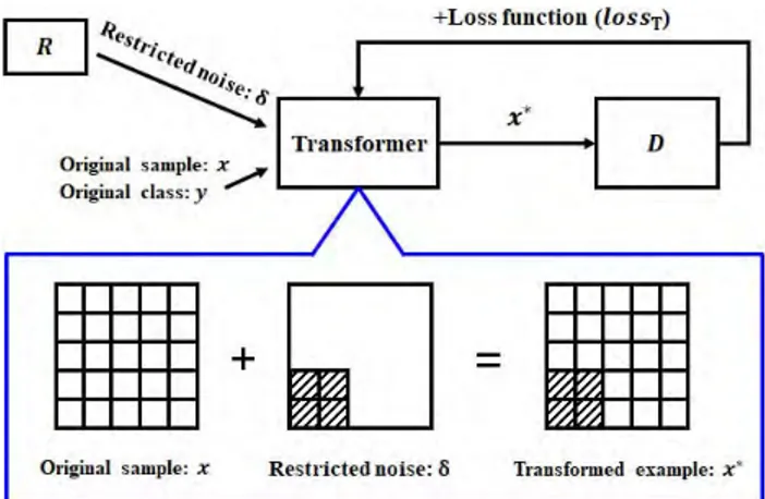
FIGURE 1. Proposed architecture. III. PROPOSED METHOD
Fig. 1 shows the proposed architecture designed to create a restricted adversarial example. The proposed architecture consists of a model D, a transformer, and a restrictor R that controls the size of the restricted pixel region. The restrictor R provides a restricted noise to the transformer by select-ing a restricted pixel area from the entire pixel image. The transformer creates a restricted adversarial example using the feedback (the loss function results) from model D.
The purpose of the proposed scheme is to generate a restricted adversarial example x⇤ that is misclassified as
the wrong class by model D while minimizing the distance between the restricted adversarial example x⇤and the original
sample x. In the mathematical expressions, the operation function of D is denoted as f (x). Given restricted noise ,
the pretrained model D, original sample x, and original class y, the transformer generates a restricted adversarial example x⇤by taking restricted noise , the original sample x, and
orig-inal class y as the input values. For this study, the transformer presented in [3] and [23] was modified as follows:
x⇤= x + . (7)
is the restricted noise modifying only the restricted pixel area chosen by the attacker; pixel areas other than the restricted area are set to a fixed value of zero. The restricted adversarial example x⇤is the sum of original sample x and
restricted noise . Model D accepts x⇤as the input value and
provides the loss result to the transformer. After calculating the total loss lossT, the transformer repeats the above
pro-cedure to create a restricted adversarial example x⇤ while
minimizing the total loss lossTfor each iteration. This total
loss is defined as follows:
lossT= lossd+ c · lossa, (8)
where lossd is the distortion function of the loss function,
lossa is the classification loss function of D, and c is the
weight value of model D and has an initial value of 1. lossdis
the distortion distance between the transformed example x⇤
and the original sample x:
lossd= | |. (9)
The distortion loss function is |x⇤ x| = | | with L0. lossa
should be minimized:
lossa= g(x⇤), (10)
where g(k) = Z(k)org max Z(k)j j 6= org , in which
org is the original class and Z(·) [3], [17] represents the probabilities of the class predictions by model D. Model D predicts the probability of the wrong class to be higher than that of the original class by optimally minimizing lossa. Algorithm 1 provides the details of the procedure.
In Algorithm 1, some discrete pixels can be selected even if the restricted pixel region is represented by the shape of [[s11:e11,s12:e12], [s21:e21,s22:e22], [s31:e31,s32:e32]] (0
sij width of sample; 0 eij height of sample; 1
i, j 3).
IV. EXPERIMENT SETUP
In the experiment performed to evaluate the proposed scheme, noise was added to the restricted pixel region using the proposed method, generating a restricted adversarial example that will be misclassified as a wrong class by model D while minimizing the distortion of the restricted example. We used the Tensorflow library [24] for machine learning, with a Xeon E5-2609 1.7-GHz server.
A. DATASETS
We used the CIFAR10 dataset [4] and the ImageNet [6] dataset. CIFAR10 consists of 10 classes of images: planes, cars, birds, cats, deer, dogs, frogs, horses, ships, and trucks.
Algorithm 1 Restricted Adversarial Example Generation Input: x F original sample y F original class F restricted noise r F number of iterations [[s11:e11,s12:e12], [s21:e21,s22:e22], [s31:e31,s32:e32]] F restricted area
Restricted adversarial example generation: org y [[s11:e11,s12:e12], [s21:e21,s22:e22], [s31:e31, s32:e32]] for r step do x⇤ x + lossd | |
lossa Z(x⇤)org max Z(x⇤)j j 6= org
lossT lossd + c ⇥ lossa
Update by minimizing the gradient of lossT
end for return x⇤
It contains color images consisting of 3072 pixels in a [32,32,3] matrix and divided into 50,000 training data and 10,000 test data. The ImageNet dataset consists of 1000 classes of images: mink, sea lion, tiger cat, zebra, etc. It contains large-scale color images divided into 1.2 million training data and 50,000 test data.
B. PRETRAINING OF MODEL
On CIFAR10, the pretrained model D is essentially a VGG19 model [25] as given in Table 10in the Appendix. The parameter configuration of the model is given in Table8
in the Appendix. After training on 50,000 training data, model D demonstrated a 91.2% accuracy rate on the 10,000 test data. On ImageNet, the pretrained model D is the Incep-tion v3 model [26]. Instead of training our own ImageNet, we used a pretrained Inception v3 network that has about 96% accuracy.
C. RESTRICTED ADVERSARIAL EXAMPLE GENERATION
To generate the restricted adversarial example, Adam [27] is used to optimally minimize the total loss with a learning rate of 0.001 and an initial constant of 0.01. Over 10,000 itera-tions, the transformer provides x⇤to model D after updating
and then receives the feedback from the model. At the end of the iterations, we evaluate the restricted example that is misclassified as a wrong class by model D.
D. RESTRICTED AREA
In order to test the performance according to the characteris-tics of the restricted area, the attack success rate and the dis-tortion of the restricted adversarial examples were evaluated by measuring them after dividing the adversarial examples
TABLE 1.Samples of restricted adversarial examples for each restricted pixel area size of square shape in bottom left position in CIFAR10 [4].
FIGURE 2. Positions and shapes of restricted areas. There are four positions: (1) top left, (2) top right, (3) bottom left, and (4) bottom right. There are three types of shapes: Square, circle, and outer-border square. (a) Positions. (b) Shapes.
into three types according to the position, shape, and size of the restricted area. As shown in Fig.2(a), the positions for the restricted area were the top left, top right, bottom left, and bottom right. The shapes of the restricted area were a square shape, a circle shape, and an outer-border square shape as shown in Fig.2(b). Finally, the sizes of the restricted area were 6%, 8%, 10%, 12%, and 14%. For example, in the case of the bottom left position and the square shape, shown in Table1, the restricted areas of attack were only a part of the [32,32,3] image as follows. The restricted areas selected for attack were [[0:8,0:8], [0:8,0:8], [0:8,0:8]], [[0:9,0:9], [0:9,0:9], [0:9,0:9]], [[0:10,0:10], [0:10,0:10], [0:10,0:10]], [[0:11,0:11], [0:11,0:11], [0:11,0:11]], [[0:12,0:12], [0:12, 0:12], [0:12,0:12]]. The sizes of the restricted areas attacked were 192, 243, 300, 363, and 432 pixels; these represent
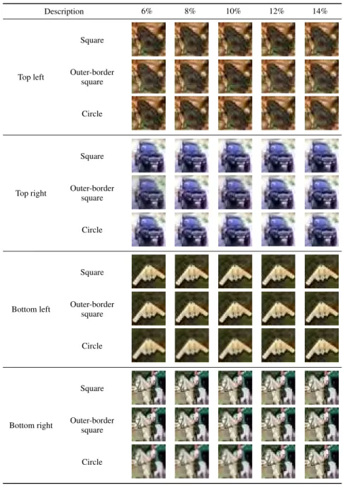
TABLE 2. Samples of restricted adversarial examples for each restricted pixel area size and position attacked in CIFAR10.
approximately 6%, 8%, 10%, 12%, and 14%, respectively, of the whole.
V. EXPERIMENTAL RESULTS
We analyzed the attack success rate, distortion, and image samples of the restricted adversarial examples by the shape, location, and size of the restricted area. The attack success rate is the discrepancy between the original class and the class output by the model. The definition of the distortion rate is the square root of the sum of each pixel’s difference from the original sample (the L2distortion measure).
Table 1 shows an example of a restricted adversarial example that is incorrectly classified as a wrong class by model D for each restricted area size attacked in CIFAR10.
Table1shows that the restricted adversarial example is mis-classified as a wrong class by the DNN but is correctly recognized by humans. Moreover, to human perception, there is little difference in the restricted adversarial examples between restricted areas of 6% and 14%.
Table2shows restricted adversarial examples for the var-ious sizes of restricted area according to the position of the restricted area (top left, top right, bottom left, or bottom right) in CIFAR10. In Table2, it can be seen that it is difficult for a human to discern the distortion of the restricted adversarial example according to the size or position of the area; this is due to the fact that they are color images. Thus, although the distortion varies according to the area restricted, a restricted adversarial example can cause misclassification by the DNN
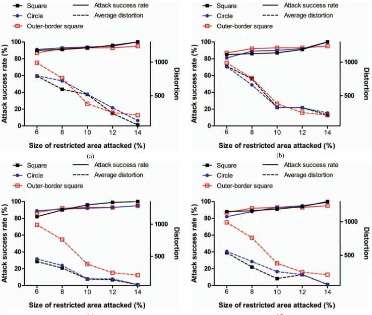
FIGURE 3. Attack success rate of the proposed method and average distortion for each restricted area size and position attacked in CIFAR10. (a) Top left position. (b) Top right position. (c) Bottom left position. (d) Bottom right position.
with minimal distortion at any position for the restricted area.
Fig. 3 shows the attack success rate and average dis-tortion for 100 random restricted adversarial examples per restricted pixel area size for each position and shape type of the restricted area in CIFAR10. As shown in the figure, as the size of the restricted area increases, the attack suc-cess rate increases because the number of attackable pixels increases. Furthermore, as the size of the restricted area increases, average distortion is reduced because the pro-posed method can more easily achieve attack success by distorting only a few pixels. Overall, when the restricted area is about 14%, the restricted adversarial examples have an attack success rate of nearly 100%. We can see that the attack success rate and distortion each differ according to the shape of the restricted area. In particular, the outer-border
square has higher distortion and a lower attack success rate than the square or the circle. Regardless of the position of the restricted area, the attack success rate of the restricted adversarial example can be seen to have a nearly identical pattern. In terms of distortion, however, it can be seen that the distortion of the restricted adversarial example varies according to the position of the restricted area. It can be seen that the required amount of distortion differs according to the position of the distortion in the original image.
The performance of the proposed method was compared with that of the state-of-the-art method, known as the Car-lini method (CW) [3], and that of the fast-gradient sign method (FGSM) [7]. FGSM, a simple and powerful attack, is a typical adversarial attack. The epsilon parameter of the FGSM was set to an initial value of 0.3. The CW method, because it is the latest method to improve performance over
TABLE 3. A sampling of the untargeted adversarial examples generated by the fast-gradient sign method (FGSM); the Carlini methods CW-L0, CW-L2, and CW-L1; and the proposed method (14% restricted area of square shape in bottom left position) on CIFAR10.
TABLE 4. Adversarial examples generated by FGSM, CW-L0, and the proposed method (1.07% restricted area of square shape in bottom left position) on ImageNet. (a) FGSM. (b) CW-L0. (c) Proposed.
the known FGSM, I-FGSM, and Deepfool method, has 100% attack success and minimal distortion. The CW method can take three forms according to the distortion function used: CW-L0, CW-L2, and CW-L1, described in SectionII.
Table3shows untargeted adversarial examples generated on CIFAR10 by the FGSM, CW-L0method, CW-L2method,
CW-L1method, and proposed scheme (14% restricted area of square shape in bottom left position). Although distortion is produced differently by each method, it can be seen in the table that it is difficult to detect with the human eye. The results displayed in the table show that the proposed method has performance similar to that of CW in terms of similarity to the original image.
Table 5 shows the average distortion and attack success rates for FGSM and the CW-L0, CW-L2, CW-L1, and
pro-posed methods on CIFAR10. As FGSM generates the adver-sarial example by taking the feedback from the target model only once, the attack success rate is somewhat lower, and greater distortion is needed. As seen in the table, in terms of average distortion, the proposed scheme produces more
TABLE 5.Comparison of FGSM, CW-L0method, CW-L2method, CW-L1 method, and proposed scheme (14% restricted area of square shape in bottom left position) on CIFAR10.
TABLE 6.The noise sampling of adversarial example ‘‘car’’ in Table3with FGSM, the CW-L0method, the CW-L2method, the CW-L1method, and the proposed scheme (14% restricted area of square shape in bottom left position) for CIFAR10.
distortion than the CW methods; this is due to its restriction on the area.
Table6shows the noise sampling of adversarial example ‘‘car’’ in Table3for FGSM, the CW-L0method, the CW-L2
method, the CW-L1 method, and the proposed scheme (14% restricted area of square shape in bottom left position) for CIFAR10. Because FGSM receives feedback from the target model only once, the adversarial example generated by FGSM has much noise, as we can see in the table. The adversarial examples generated by the CW-L0 method, the
CW-L2method, and the CW-L1method cause
misinterpre-tation by the target model by modulating the pixels that have a large influence on the misclassification of the entire image. Under the proposed method, noise is added only within a defined restricted area; no noise is added to other areas. Thus, the conventional methods add noise to the whole area of the original image; the proposed method, in contrast, adds noise only in the restricted area, which is not easily recognizable to the human eye.
In order to show the performance of the proposed method on other datasets, we measured the performance of the proposed method on ImageNet data. Restricted adversar-ial examples were generated by modulating restricted areas [0:40, 0:50, 3] (modifying only 1.07% of the total image). Table4shows a sampling of the adversarial examples gen-erated by FGSM, CW-L0, and the proposed method (1.07%
restricted area of square shape in bottom left position) on ImageNet. The original sample is classified as frying pan, and the adversarial example generated by each method is incorrectly classified as pizza. As shown in Table7, the pro-posed method has a 100% attack success rate even after changing an area restricted to only about 1.07% for 100 ran-dom samples. Table 4 and Table 7 show that, as with the CIFAR10 results, FGSM adds more distortion than the other methods, which is because it receives feedback only once. Although the proposed method produces a more distorted image than the CW-L0method, which adds distortion to the
entire image, the proposed method adds the noise only in a limited area, making it difficult for humans to perceive, and it shows high performance. Because ImageNet images have many more pixels than CIFAR10 images, the proposed method has particularly good performance on ImageNet even if the restricted area is small.
TABLE 7. Comparison of FGSM, CW-L0method, and proposed scheme (1.07% restricted area of square shape in bottom left position) on ImageNet [6].
VI. DISCUSSION
A. ASSUMPTION
The proposed scheme assumes a white box attack, in which the attacker has detailed information about the target model. By adding a little noise to a restricted area of the original sample, the proposed method is optimized to satisfy both the minimal distortion and the attack success requirements. Thus, the proposed method can create restricted adversarial
FIGURE 4. Computation time to generate restricted adversarial examples for basic CNN, VGG19 model [25], and distillation method.
examples for a 100% success rate against the target model with the appropriate 14% and 1.07% restricted areas in CIFAR10 and ImageNet, respectively.
B. AREA OF RESTRICTION
The proposed method offers the advantage of controlling the size, shape, and position of the restricted pixel region. We evaluated the attack success rate, distortion, and image samples of restricted adversarial examples by adjusting the size, shape, and position of the restricted area. The evaluation showed that the distortion in the restricted area was so small it could not be identified by eye. Although the restricted pixel area is a specific part of the image, the restricted adversarial example is difficult for humans to detect, and it causes mis-classification by the DNN.
C. ATTACK CONSIDERATIONS
The proposed method is a white box attack using the modified Carlini method [3]. It can control the amount of distortion and the attack success rate. The proposed method is an untar-geted attack and requires more process iterations to generate restricted adversarial examples. The attack success rate varied according to the size, shape, and position of the restricted area. To achieve an attack success rate of 100%, the method requires an appropriate restricted pixel area size. When the restricted pixel area size in the experiment was approximately 14% in CIFAR10 and 1.07% in ImageNet, the proposed method achieved a 100% success rate.
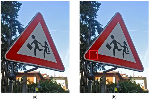
The restricted adversarial example can be used with appli-cations such as stickers. For example, when road signs have already been deployed, the proposed method can be used by applying a sticker to a sign. Fig.5in the Appendix shows an original road sign and a restricted road sign in which only a restricted area has been modified. The image size is [375,500,3], and restricted adversarial examples were gen-erated by modulating a specific area of the sign ([54:98, 272:317, 3]) (modifying only 1.2% of the total image). The original sample was correctly classified as a street sign, but the restricted adversarial example was mistakenly classified as a church. Whereas humans will not detect the change in
FIGURE 5. A restricted adversarial example for an original sample of a road sign in ImageNet. (a) Original sample. (b) Restricted adversarial example.
a road sign with such a sticker, the sign will be incorrectly classified as a wrong class by DNNs.
In addition, the restricted adversarial example can be used for face recognition data. It can be used to cause a false recognition by modulating a specific area of the face. The model used was pretrained Inception-ResNet-v1 [28], and the dataset used was Labeled Faces in the Wild (LFW) [29]. Fig.6in the Appendix shows a sampling of restricted adver-sarial examples generated for the original sample in the LFW dataset. The image size was [250,250,3], and restricted adver-sarial examples were generated by modulating pixels within a specific area of the sign ([135:145, 75:85, 3], modifying only 0.19% of the total image). The original sample was correctly classified as Ana Paula Gerar, but the restricted adversarial example was mistakenly classified as Candle Kung. This method may be used to mislead a face recognition system by applying makeup to a specific area on a human’s face.
D. COMPUTATION COST
In order to compare the computation costs, we tested the per-formance on the CIFAR10 dataset with a basic convolutional neural network (CNN) model (Table 9 in the Appendix), a distillation method [8] with adversarial example defense, and a deeper CNN model, the VGG19 model [25] (Table10in the Appendix). This defensive distillation method [8] has two neural networks, in which the output class probability of the classifier is used as the input for the second stage of classifier training. In the distillation method, we used two basic DNN models (Table9in the Appendix). We created 100 restricted adversarial examples for each model and measured compu-tation space and compucompu-tation time as compucompu-tation cost. The restricted area is the 14% restricted area of square shape in the bottom left position. In terms of computation space, the basic
CNN model was 9.2 MB, the VGG19 model was 312.1 MB, and the distillation model was 18.4 MB. In terms of computa-tion time, Fig.4in the Appendix shows the computation time needed to generate 100 restricted adversarial examples for the basic CNN, VGG19 model, and distillation method, when the attack success rate is 100%. As shown in the figure, the com-putation time needed to generate the restricted adversarial examples remains nearly constant across changes in the size of the restricted area. On the other hand, the more complex the model is, the more computation time is required depending on the characteristics of the model. In particular, if the target model is a defense system, more computation time is needed. Although the target model is complex, the proposed method has a 100% attack success rate because it is a white box method.
E. DISTORTION
There is a trade-off between the distortion and the area of restriction. When generating restricted adversarial exam-ples, the attacker must consider this trade-off. For example, the restricted adversarial example generated by the proposed method is somewhat more distorted than an adversarial exam-ple generated by the Carlini method. This is because if distor-tion is applied in a limited area of the image rather than in the entire image, the number of attackable pixels will be smaller. However, although the method of distorting the limited image region increased the distortion somewhat, it maintained the rate of human perception to a level similar to that of the original sample because it was performed on a color image. VII. CONCLUSIONS
In this study, we proposed a restricted adversarial example for which only a part of an image is modified. The restricted adversarial example will be misclassified as a wrong class by
FIGURE 6. A restricted adversarial example for an original sample in the LFW [29] dataset. (a) Original sample. (b) Restricted adversarial example.
TABLE 8. Model parameters.
TABLE 9. Basic CNN model.
model D while maintaining a minimum distortion distance from the original sample. To evaluate the performance of the proposed scheme, we analyzed restricted adversarial exam-ples, the restricted pixel area size, the restricted pixel area shape, the restricted pixel area position, the attack success rate, and average distortion. The results show that the pro-posed scheme can generate a restricted adversarial example with a 100% attack success rate with a restricted pixel region of the whole (approximately 14% for CIFAR10 and 1.07% for ImageNet).
Future research will extend the experiment to other stan-dard datasets, such as those for voice and video domains. In addition, the concept of the proposed scheme can be applied to CAPTCHA systems [30]. We can also work on developing a restricted adversarial example method such as that used in the generative adversarial net [13] instead of
TABLE 10.Target model architecture [25] for CIFAR10.
using transformation. Finally, developing a defense against the proposed scheme will be another challenge.
APPENDIX
See Tables 8–10 and Figs. 4–6. ACKNOWLEDGMENT
The authors would like to thank the editors and the anony-mous reviewers, who gave us very helpful comments that improved this paper.
REFERENCES
[1] J. Schmidhuber, ‘‘Deep learning in neural networks: An overview,’’ Neural Netw., vol. 61, pp. 85–117, Jan. 2015.
[2] C. Szegedy et al., ‘‘Intriguing properties of neural networks,’’ in Proc. 2nd Int. Conf. Learn. Represent. (ICLR), Banff, AB, Canada, Apr. 2014. [Online]. Available: http://arxiv.org/abs/1312.6199
[3] N. Carlini and D. Wagner, ‘‘Towards evaluating the robustness of neu-ral networks,’’ in Proc. IEEE Symp. Secur. Privacy (SP), May 2017, pp. 39–57.
[4] A. Kurakin, I. J. Goodfellow, and S. Bengio, ‘‘Adversarial examples in the physical world,’’ in Proc. 5th Int. Conf. Learn. Represent. (ICLR), Toulon, France, Apr. 2017. [Online]. Available: https://openreview.net/forum?id=HJGU3Rodl
[5] S.-M. Moosavi-Dezfooli, A. Fawzi, and P. Frossard, ‘‘DeepFool: A simple and accurate method to fool deep neural networks,’’ in Proc. IEEE Conf. Comput. Vis. Pattern Recognit., Jun. 2016, pp. 2574–2582.
[6] J. Deng, W. Dong, R. Socher, L.-J. Li, K. Li, and L. Fei-Fei, ‘‘ImageNet: A large-scale hierarchical image database,’’ in Proc. IEEE Conf. Comput. Vis. Pattern Recognit. (CVPR), Jun. 2009, pp. 248–255.
[7] I. J. Goodfellow, J. Shlens, and C. Szegedy, ‘‘Explaining and har-nessing adversarial examples,’’ in Proc. 3rd Int. Conf. Learn. Repre-sent. (ICLR), San Diego, CA, USA, May 2015. [Online]. Available: http://arxiv.org/abs/1412.6572
[8] N. Papernot, P. McDaniel, X. Wu, S. Jha, and A. Swami, ‘‘Distillation as a defense to adversarial perturbations against deep neural networks,’’ in Proc. IEEE Symp. Security Privacy (SP), May 2016, pp. 582–597. [9] A. Fawzi, O. Fawzi, and P. Frossard, ‘‘Analysis of classifiers’ robustness
to adversarial perturbations,’’ Mach. Learn., vol. 107, no. 3, pp. 481–508, 2018.
[10] G. Jin et al., ‘‘APE-GAN: Adversarial perturbation elimination with GAN,’’ in Proc. IEEE Int. Conf. Acoust., Speech Signal Process. (ICASSP), 2019, pp. 3842–3846.
[11] W. Xu, D. Evans, and Y. Qi. (2017). ‘‘Feature squeezing: Detecting adversarial examples in deep neural networks.’’ [Online]. Available: https://arxiv.org/abs/1704.01155
[12] D. Meng and H. Chen, ‘‘MagNet: A two-pronged defense against adver-sarial examples,’’ in Proc. ACM SIGSAC Conf. Comput. Commun. Secur., 2017, pp. 135–147.
[13] I. Goodfellow et al., ‘‘Generative adversarial nets,’’ in Proc. Adv. Neural Inf. Process. Syst., 2014, pp. 2672–2680.
[14] N. Papernot, P. McDaniel, I. Goodfellow, S. Jha, Z. B. Celik, and A. Swami, ‘‘Practical black-box attacks against machine learning,’’ in Proc. ACM Asia Conf. Comput. Commun. Secur., 2017, pp. 506–519.
[15] G. L. Oliveira, A. Valada, C. Bollen, W. Burgard, and T. Brox, ‘‘Deep learning for human part discovery in images,’’ in Proc. IEEE Int. Conf. Robot. Autom. (ICRA), May 2016, pp. 1634–1641.
[16] F. Tramèr, N. Papernot, I. Goodfellow, D. Boneh, and P. McDaniel. (2017). ‘‘The space of transferable adversarial examples.’’ [Online]. Available: https://arxiv.org/abs/1704.03453
[17] N. Papernot, P. McDaniel, S. Jha, M. Fredrikson, Z. B. Celik, and A. Swami, ‘‘The limitations of deep learning in adversarial settings,’’ in Proc. IEEE Eur. Symp. Secur. Privacy (EuroS&P), Mar. 2016, pp. 372–387.
[18] H. Kwon, Y. Kim, K.-W. Park, H. Yoon, and D. Choi, ‘‘Multi-targeted adversarial example in evasion attack on deep neural network,’’ IEEE Access, vol. 6, pp. 46084–46096, 2018.
[19] H. Kwon, Y. Kim, K.-W. Park, H. Yoon, and D. Choi, ‘‘Friend-safe evasion attack: An adversarial example that is correctly recognized by a friendly classifier,’’ Comput. Secur., vol. 78, pp. 380–397, Sep. 2018.
[20] M. Sharif, S. Bhagavatula, L. Bauer, and M. K. Reiter, ‘‘Accessorize to a crime: Real and stealthy attacks on state-of-the-art face recognition,’’ in Proc. ACM SIGSAC Conf. Comput. Commun. Secur., 2016, pp. 1528–1540. [21] T. B. Brown, D. Mané, A. Roy, M. Abadi, and J. Gilmer. (2017).
‘‘Adver-sarial patch.’’ [Online]. Available: https://arxiv.org/abs/1712.09665 [22] J. Su, D. V. Vargas, and K. Sakurai, ‘‘One pixel attack for fooling deep
neural networks,’’ IEEE Trans. Evol. Comput., to be published. [23] F. Zhang, P. P. K. Chan, B. Biggio, D. S. Yeung, and F. Roli, ‘‘Adversarial
feature selection against evasion attacks,’’ IEEE Trans. Cybern., vol. 46, no. 3, pp. 766–777, Mar. 2016.
[24] M. Abadi et al., ‘‘TensorFlow: A system for large-scale machine learning,’’ in Proc. OSDI, vol. 16, 2016, pp. 265–283.
[25] K. He, X. Zhang, S. Ren, and J. Sun, ‘‘Deep residual learning for image recognition,’’ in Proc. IEEE Conf. Comput. Vis. Pattern Recognit., Jun. 2016, pp. 770–778.
[26] C. Szegedy, V. Vanhoucke, S. Ioffe, J. Shlens, and Z. Wojna, ‘‘Rethinking the inception architecture for computer vision,’’ in Proc. IEEE Conf. Comput. Vis. Pattern Recognit., Jun. 2016, pp. 2818–2826.
[27] K. J. Geras and C. A. Sutton, ‘‘Scheduled denoising autoencoders,’’ in Proc. 3rd Int. Conf. Learn. Represent. (ICLR), San Diego, CA, USA, May 2015. [Online]. Available: http://arxiv.org/abs/1406.3269
[28] C. Szegedy, S. Ioffe, V. Vanhoucke, and A. A. Alemi, ‘‘Inception-v4, inception-resnet and the impact of residual connections on learning,’’ in Proc. 31st AAAI Conf. Artif. Intell., 2017, pp. 4278–4284.
[29] E. Learned-Miller, G. B. Huang, A. RoyChowdhury, H. Li, and G. Hua, ‘‘Labeled faces in the wild: A survey,’’ in Advances in Face Detection and Facial Image Analysis. Springer, 2016, pp. 189–248. [Online]. Avail-able: https://www.springerprofessional.de/en/labeled-faces-in-the-wild-a-survey/9975982
[30] M. Osadchy, J. Hernandez-Castro, S. Gibson, O. Dunkelman, and D. Pérez-Cabo, ‘‘No bot expects the deepCAPTCHA! Introducing immutable adversarial examples, with applications to CAPTCHA genera-tion,’’ IEEE Trans. Inf. Forensics Security, vol. 12, no. 11, pp. 2640–2653, Nov. 2017.
HYUN KWON received the B.S. degree in mathematics from Korea Military Academy, South Korea, in 2010, and the M.S. degree from the School of Computing, Korea Advanced Institute of Science and Technology (KAIST), in 2015, where he is currently pursuing the Ph.D. degree. His research interests include computer security, infor-mation security, and intrusion-tolerant systems.
HYUNSOO YOON received the B.E. degree in electronics engineering from Seoul National Uni-versity, South Korea, in 1979, the M.S. degree in computer science from the Korea Advanced Insti-tute of Science and Technology (KAIST), in 1981, and the Ph.D. degree in computer and information science from Ohio State University, Columbus, OH, USA, in 1988. From 1988 to 1989, he was a Member of the Technical Staff with AT&T Bell Labs. He is currently a Professor with the School of Computing, KAIST. His research interests include 4G networks, wireless sensor networks, and network security.
DAESEON CHOI received the B.S. degree in computer science from Dongguk University, South Korea, in 1995, the M.S. degree in com-puter science from the Pohang Institute of Sci-ence and Technology, South Korea, in 1997, and the Ph.D. degree in computer science from the Korea Advanced Institute of Science and Tech-nology, South Korea, in 2009. He is currently a Professor with the Department of Medical Infor-mation, Kongju National University, South Korea. His research interests include identity management and information security.
![TABLE 1. Samples of restricted adversarial examples for each restricted pixel area size of square shape in bottom left position in CIFAR10 [4].](https://thumb-ap.123doks.com/thumbv2/123dokinfo/5089031.76414/5.864.444.809.129.729/table-samples-restricted-adversarial-examples-restricted-square-position.webp)
![FIGURE 4. Computation time to generate restricted adversarial examples for basic CNN, VGG19 model [25], and distillation method.](https://thumb-ap.123doks.com/thumbv2/123dokinfo/5089031.76414/9.864.102.371.872.929/figure-computation-generate-restricted-adversarial-examples-distillation-method.webp)
![FIGURE 6. A restricted adversarial example for an original sample in the LFW [29] dataset](https://thumb-ap.123doks.com/thumbv2/123dokinfo/5089031.76414/11.864.188.676.96.347/figure-restricted-adversarial-example-original-sample-lfw-dataset.webp)
