Physical and Particle Flow Modeling of Shear Behavior of
Non-Persistent Joints
A. Ghazvinian1, V. Sarfarazi2, H. Nejati2 and M. R. Hadei2
1Academic Member, Rock Mechanics Division, Tarbiat Modares University, Tehran, Iran 2Research Scholar, Rock Mechanics Division, Tarbiat Modares University, Tehran, Iran
Abstract
Laboratory experiments and numerical simulations using Particle Flow Code (PFC2D) were performed to study the effects of joint separation and joint overlapping on the full failure behavior of rock bridges under direct shear loading. Through numerical direct shear tests, the failure process is visually observed and the failure patterns are achieved with reasonable conformity with the experimental results. The simulation results clearly showed that cracks developed during the test were predominantly tension cracks. It was deduced that the failure pattern was mostly influenced by both of the joint separation and joint overlapping while the shear strength is closely related to the failure pattern and its failure mechanism. The studies revealed that shear strength of rock bridges are increased with increasing in the joint separation. Also, it was observed that for a fixed cross sectional area of rock bridges, shear strength of overlapped joints are less than the shear strength of non-overlapped joints.
Key words: Non-persistent joint, rock bridge, joint separation, joint overlapping, shear fracture.
1. Introduction
Rock masses are usually discontinuous in nature due to various geological processes and only in few cases geometry of a rock failure is limited to a single discontinuity [1]. Besides the discontinuities themselves, regions between adjacent discontinuities (rock bridges) are of utmost importance in rock mass failure [2, 3]. Initiation, propagation and coalescence of non-persistent joints are important factors in controlling the mechanical behavior of rock structures such as slopes, foundations and tunnels. Therefore, a comprehensive study on the shear failure behavior of rock bridges can provide an in depth understanding of both local and general rock instabilities, leading to an improved design for rock engineering projects.
The failure behavior of jointed rock under shear loading has drawn much attention from both researchers and practical engineers over the last three decades and some extensive works on the coalescence pattern and shear resistance have been carried out through a large number of experimental and theoretical studies. In one of the pioneering works done by Lajtai [4,5], tensile wing cracks were found to first appear at the tips of horizontal joints, followed by the secondary shear cracks propagating towards the opposite joint. Savilahti et al. [6] did some further study on the specimens of jointed rock under direct shear tests where the joint separation varies in both horizontal and vertical directions and joint arrangement changes from non-overlapping to overlapping using modeling material. The coalescence patterns for the specimens indicated that the jointed rock is failed in mixed mode for non-overlapping joint and in tensile mode for overlapping joint. Wong et al. [7] studied shear strength and failure pattern in models containing arrayed open joints in both modeling plaster material and natural rocks under direct shear tests. The results showed that failure pattern was mainly controlled by the joint separation while shear strength was mostly influenced by the failure pattern. Ghazvinian et al. [8] made a thorough study in shear behavior of the rock-bridges based on the changes in their persistency and cross sectional area. The analysis proved/showed that the failure mechanism is influenced by rock-bridges consistency. Gehle and Kutter’s [9] investigation on the breakage and shear behavior of intermittent rock joints, under direct shear loading condition, showed that joint orientation is an important influential parameter for shear strength of jointed rock. It should be noted that the equivalent material modeling results are very sensitive to sample preparation, loading conditions. Also, in the physical modeling, failure mechanism cannot be traced [10]. To overcome the weaknesses of the physical modeling, numerical modeling can be implemented. By numerical approach, problems with high mechanical and geometrical complexity can easily be simulated. In this regard, several numerical techniques such as finite element method (FEM) [11], boundary element method (BEM) [12-14] and displacement discontinuity method (DDM) are being used.
During the past decades, numerous theories for predicting stress distribution and crack propagation have
been proposed. For most practical purposes, three fundamental theories commonly employed [15] are maximum tangential stress theory [16], maximum energy release rate theory [17] and minimum energy density theory [18]. These theories are only applicable for prediction of tensile crack initiation and for shear crack initiation another approach should be utilized [15]. The Damage Model of Reyes and Einstein [19] and the F-criterion of Shen and Stephansson [20] have been specifically developed for crack coalescence through shear cracks. However, both the models have been successfully used only in uniaxial compression tests [15]. Bobet and Einstein proposed a new analytical criterion for both wing and secondary shear cracks [21]. This criterion is based on the assumption that crack initiation depends on the state of the stress rather than on the stress intensity factor (SIF).
Various investigations have been carried out on the simulation of crack propagation and coalescence in models with multiple cracks. Scavia and Castelli [22] and Scavia [23] have conducted some preliminary work using numerical modeling based on DDM to investigate the mechanical behavior of rock bridges in material containing two and three crack-like flaws. They concluded that direct and induced tensile crack propagation occurs in either stable or unstable conditions depending on flaw spacing and applied confining stresses. Vasarhelyi and Bobet [15] also used DDM to model failure mechanism between two bridged flaws in gypsum under uniaxial compression. Their simulations reproduced the types of coalescence observed in the experiments, and predicted an increase in coalescence stresses with ligament length.
It is noted that in the aforesaid studies simulation of the shear response in the specimens containing non-persistent joint under direct shear test has not been considered. In this paper, an attempt has been made to apply 2D Particle flow code for investigating the effect joint separation and joint overlapping on the shear behavior of rock bridges.
2. Laboratory tests and results
2.1. Model material preparation
The model material used in preparing the intact samples and jointed blocks was a combination of plaster 37.5%, cement 25%, and Water 37.5%.
The process of mixing of the material constituents were carried out with an electric blender. To ensure material homogeneity, plaster of Paris and cement were initially mixed. Subsequently, water was added to the constituents and thoroughly re-mixed and casted in molds with different shapes and volumes. The samples were then taken out of the mold, and kept in the geomechanics laboratory room with constant temperature of 20±2 °C for 20 days. The mold dimension for cylindrical sample was 54 mm in diameter
and 108 mm in length. The mold dimension for disc sample was 54 mm in diameter and 27 mm in thickness (Fig. 1a).
(a) (b)
Fig.1. a) two different molds used for the fabrication of the cylindrical samples, b) model used for the fabrication of the jointed specimens.
2.2. Intact model material properties
The uniaxial, triaxial compression and Brazilian tensile tests were performed by MTS machine to determine the mechanical properties of the intact model material. The mechanical properties of the physical models are summarized in Table 1.
Table 1. Experimentally determined property values of intact model material.
Property value Average uniaxial compressive strength (MPa) 6.6
Average Brazilian tensile strength (MPa) 1
Average Young’s Modulus in compression (GPa) 5
Average Poisson’s ratio 0.18
Internal angle of friction 20.4°
Cohesion (MPa) 2.2
2.3. Preparation, testing and results of models possessing
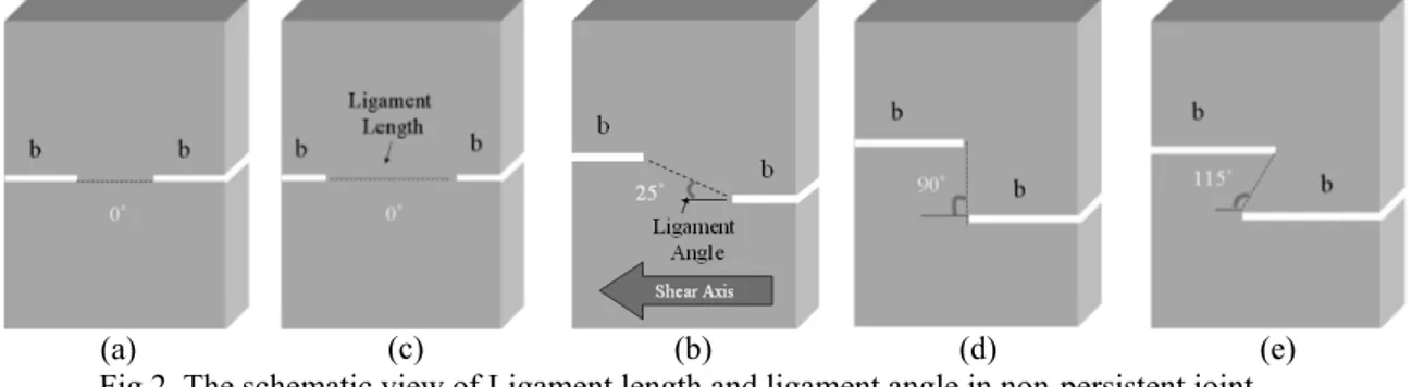
The procedure developed by Bobet [24] for preparing open non-persistent joints was used in this research with some modifications. The mold dimension for discontinuous jointed samples was 190 mm in length, 150mm in width and 50 mm in thickness. The mold consists of four fiberglass sheets bolted together and of two fiberglass plates, with thickness of 20 mm, which are placed at the top and bottom of the mold (Fig 1.b). The top plate has two orifice openings used to fill the mold with the liquid mixture. The upper and the lower surfaces have slits cut into them. The opening of slits is 1 mm and their tract is equal to the width of the model. The depths of slits in upper and lower sheets are 20 mm and 10 mm, respectively. Using these slits, greased metallic shims are inserted in the mold to produce non-persistent joints. Fabricated sample was kept in the mold for about seven hours. Then the specimens were un-molded and the metallic shims pulled out of the specimens. A total of five specimens containing planar and echelon persistent joints were prepared and tested. Two of the specimens were containing two planar non-persistent joints with different ligament lengths i.e. 45mm and 90mm. Ligament length was defined as distance between the tips of two joints (Fig. 2a, b). For different specimens, the lengths of edge joints were different. The joint lengths (b) in two different samples were kept 52.5 and 30 mm, respectively. Three of the fabricated specimens were containing two echelon non-persistent joints with similar ligament length (45 mm) with varying ligament angle of 25°, 90° and 115°, (Fig.2). It is to note that ligament angle
was defined as the angle between the ligament and shear axis. The angles were measured counter-clockwise from the shear axis (Fig. 2c, d, e). For different specimens, the lengths of edge-notched joints were different. The joint lengths (b) were 66.8, 75 and 78.8 mm which were associated with ligament angles of 25°, 90° and 115°, respectively.
(a) (c) (b) (d) (e)
Fig 2. The schematic view of Ligament length and ligament angle in non-persistent joint.
Based on the variation in the joint length, it was possible to define the joint coefficient (JC) as the ratio of the joint length to the total shear length. The values of ligament length, joint length and joint coefficient of fabricated models are listed in Table 2.
Table 2. The values of joint length and ligament length in different models. Ligament angle Ligament length (l) (mm) Joint length (b) (mm) JC
0° 45 52.5 0.7
0° 90 30 0.4
25° 45 66.8 0.71
90° 45 75 0.77
A servo-controlled MTS direct shear apparatus, shown in Fig 3, was used for the purpose of testing artificial non-persistent joints.
Fig 3. Photograph of shear testing device.
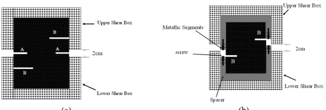
The gap distance between the upper and lower shear boxes was equal to 2 cm, therefore only one horizontal failure surface could exist in the physical model. It means that, it was only possible to perform the shear test on the planar non-persistent joint set AA while the shear test on the echelon joint set BB was accompanied with technical problem due to non-flexibility in gap distance between the shear boxes (Fig 4a). To overcome this problem, the spacers made from several screwed metallic segments were inserted between the sample and shear box (Fig. 4b). The numbers of these segments were possible to be changed to make a desirable gap between the spacers based on the joint position. This arrangement provided considerable flexibility for evaluating the shear behavior of echelon non-persistent joints.
(a) (b)
Fig. 4. Schematic view of shear box. a) General shear box; b) Modified shear box.
All samples were tested by applying a shear displacement rate of 0.01mm/s. the normal stress applied to the rock bridges was 0.33 MPa which is approximately 5% of uniaxial strength of intact sample. The shear loads as well as the shear displacements are taken by a data acquisition system during the shear test. The crack pattern is observed after the test is completed. It was observed, after the test, that the pre-existing joint surfaces have not been destroyed during the test. It means that the rock joint has not any effect on the shear behavior of rock bridge. The shearing process of a discontinuous joint constellation begins, as one would expect, with the formation of new fractures which eventually transect the material bridges and lead to a through-going discontinuity. The observation results show that the both of the joint separation and joint overlapping influence the failure pattern of rock bridge. Figure 5 shows five different types of failure pattern obtained in direct shear tests.
I) Failure pattern in planar non-persistent joint (Ligament angle is 0°)
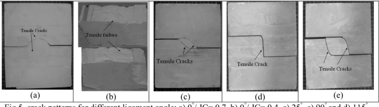
When ligament length is 45mm (fig 5.a), the upper tensile crack propagate through the intact portion area but the lower tensile crack develops for a short distance, and then becomes stable so as not to coalesce with the tip of other joint.
When ligament length is 90mm (fig 5.b), interaction between the joint is not strong so that the tensile cracks propagates in the mid zone. In this case, the rock bridge is broken with an uneven failure surface.
(a) (b) (c) (d) (e) Fig 5. crack patterns for different ligament angle; a) 0°/ JC= 0.7, b) 0°/ JC= 0.4, c) 25°, c) 90° and d) 115°.
When ligament angle was 25° (fig 5.c), the wing cracks were initiated at the tip of the joints and
propagated in curvilinear path until coalescing with the tip of the other joint. This coalescence left an elliptical core completely detached from the sample.
When ligament angle was 90° (fig 5.d), the tensile crack was initiated at the joint tip and propagated
through the bridged segment. In this configuration, the rock bridge was broken with a single failure surface.
When ligament angle was 115° (fig 5.e), the wing cracks were initiated at the joint walls and developed
almost in a vertical direction. These wing cracks propagated through the intact portion area till coalescing with the opposite joint tips. This coalescence also left an elliptical core of intact material completely detached from the sample.
All of the introduced failure patterns were tensile as there were no crushed or pulverized materials available at the failure location and also there were no evidence of shear movement.
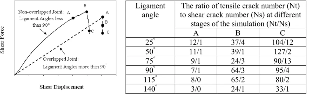
The shear stress and horizontal displacement measured for each ligament angle is illustrated in Fig. 6. It was noticed that the non-overlapped joints (ligament angles less than 90°) exhibited non-linear behavior
under direct shear loading while the overlapped joints have a linear behavior.
Fig 6 depicts that when ligament length were 45mm, the shear loading capacity of non-overlapped joints were more than the shear loading capacity of overlapped joints due to normal load appearances on the rock bridge in non-overlapped joint configuration. Also, the loading capacities were increased with increasing the ligament length.
Fig.6. Shear force versus shear displacement curves for different ligament angles.
In simulation of bonded particle model by PFC2D, rock material is represented as an assembly of circular disks bonded together at their contact points and confined by planar walls. There are two basic bonding models supported in PFC: contact-bonded model and parallel-bonded model. A contact bond approximates the physical behavior of a small cement-like substance lying between particles. In fact, the contact bond behaves as a parallel bond of radius zero. A contact bond does not have shear and normal stiffness and therefore cannot resist a bending moment. In the simulation process, the contacts bonds are assigned with specified tensile and shear strength. The details of PFC software are well described by [25, 26].
In order to generate a contact-bonded particle model the micro parameters including ball-to-ball contact modulus, stiffness ratio kn over ks, ball friction coefficient, contact normal bond strength, contact shear bond strength, ratio of standard deviation to mean of bond strength both in normal and shear direction, and minimum Ball radius have to be determined. In this study, a parallel-bonded particle model which is a modification of contact-bonded particle model with three additional micro parameters (i.e., parallel-bond radius multiplier, parallel-bond modulus, and parallel-bond stiffness ratio).
The parameters governing the particle contact properties and bonding characteristics cannot be determined directly from tests performed on laboratory model samples. For this, an inverse modeling procedure was used for determining the appropriate micro-mechanical properties of the numerical models from the macro-mechanical properties determined in the laboratory tests [25]. With a try and error procedure, micro-mechanical properties are chosen and accordingly macro mechanical properties are estimated. The micro-mechanical properties which provide macroscopic response close to that of the laboratory tests are then adopted for the jointed blocks.
3.1. Preparing and calibrating the numerical model
As it was described in detail by Itasca [25], the standard process of generating a PFC2D assembly to represent a test model is used in this article. This process involves the following steps: particle generation, packing the particles, isotropic stress installation (stress initialization), floating particle (floater) elimination and bond installation. The unconfined compressive test, the Brazilian test and the biaxial test were carried out to calibrate the properties of particles and parallel bonds in bonded particle model. The applied loading rate should be properly set to ensure that the force, displacement; velocity and acceleration do not propagate farther than immediate neighboring particles during a single time step. Under the low loading rate, the sample remains in quasi-static equilibrium throughout the test.
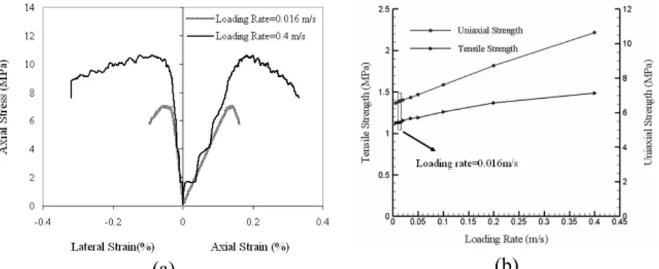
Figure 7.a shows the effect of the loading rate on the curve of axial stress versus axial strain. The mechanical responses of test samples are clearly dependent on the loading rate in the elastic range. In the case of loading rate of 0.4 m/s, an oscillatory behavior in the stress-strain curve is occurred. The oscillatory behavior of the mechanical response is greatly reduced when the smaller loading rate (i.e. 0.016 m/s) is used in the simulation.
(a) (b)
Figure 7. The effect of the loading rate on the: a) curve of axial stress versus axial strain, b) mechanical properties of numerical model.
Figure 7.b shows the effect of the loading rate on both of the uniaxial strength and Brazilian tensile strength of numerical model. As it can be seen, the compressive and tensile strength are remained constant in the loading rate of ‘0.016 m/s’. Therefore, this loading rate was applied in all of the simulations.
Using the standard calibration procedures [25], a calibrated PFC particle assembly was created. The micro-properties were listed in Table 3.
Table 3. Micro properties used to represent intact rock
Parameters Values Parameters Values
Type of particles Disc Parallel-bond radius multiplier 1
Density (kg/m3) 1000 Young’s modulus of parallel bond (GPa) 4
Minimum radius (mm) 0.27 Parallel bond stiffness ratio 1.7
Size ratio 1.56 Particle friction coefficient 0.4
porosity 0.08 Parallel bond normal strength, mean (MPa) 5.6
Damping ratio 0.7 Parallel bond normal strength, std. dev. (MPa) 1.4
Contact Young’s modulus (GPa) 4 Parallel bond shear strength, mean (MPa) 5.6
Stiffness ratio 1.7 Parallel bond shear strength, std. dev. (MPa) 1.4
Fig.8. Unconfined compressive test (cracks described by red/black lines).
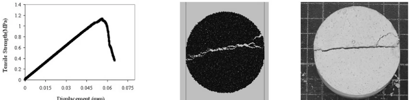
Fig 9. a) Tensile strength versus axial displacement curve for numerical Brazilian test simulation, b) failure pattern in PFC2D model, c) failure pattern in physical sample.
Fig.10.Calibrated failure locus for PFC synthetic rock compared to the Laboratory measured. As the numerical results agreed with experimental measurements, it was concluded that the assembly constructed in PFC2D could realistically represent the mechanical behavior of a rock like material. Therefore, the parameters used for the above numerical tests, which was listed in Table 3, could be introduced in the subsequent modeling of shear behavior of non-persistent joint.
3.2. Numerical direct shear test on the non-persistent open joint 3.2.1. Preparing the model
After calibration of PFC2D, direct shear tests for jointed rock were numerically simulated by creating a shear box model in PFC2D (by using the calibrated micro parameters) (Fig.11). The PFC specimen has the cross sectional dimensions of 76×60 mm. These dimensions were scaled down by 40% to reduce the running time. A total of 11179 disks with a minimum radius of 0.27 mm were used to construct the specimen. A band of the material was cut from the top and bottom of the numerical specimens in order to simulate direct shear of planar and echelon non-persistent joints.
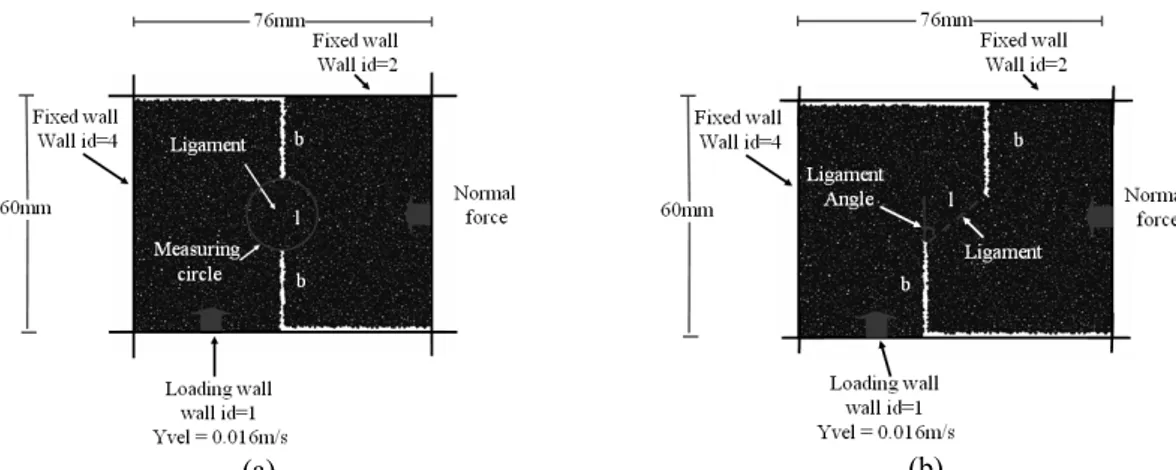
Figure 11 (a & b) demonstrates the geometry, boundary and loading conditions. Details of the simulations and conducted tests are as follows:
(a) (b)
Fig.11. Illustration of direct shear test simulation scheme in PFC; a) planar non-persistent joints, b) Echelon non-persistent joints.
I) Models with planar non-persistent joints:
Four specimens with two planar joints possessing different lengths were considered (fig. 11a). Various proportions of joint lengths were applied to investigate their effect. Based on the joint length variation, Joint Coefficient (JC) was defined as the ratio of the joint length to the shear failure length. JC was increased from 0.4 to 0.85 with increment of 0.15. It should be noted that JC was kept the same for both the numerical and physical models.
II) The models with echelon non-persistent joints:
Six specimens with two echelon joints with various ligament angles were established to investigate the influence of joint overlapping on shear behavior of rock bridges (Fig. 11b). Various proportions of joint ligament angles were applied for a parametric study. The values of joint length, ligament length and JC for different models are listed in Table 4.
Table 4. The values of joint length and ligament length in different models. Ligament
angle Ligament length (l) (mm) Joint length (b) (mm) JC
0° 9 25.5 0.85 0° 18 21 0.7 0° 27 16.5 0.55 0° 36 12 0.4 25° 18 21.8 0.71 50° 18 24.2 0.729 75° 18 27.7 0.755 90° 18 30 0.77 115° 18 33.8 0.79 140° 18 36.9 0.804
4. Discussion
4.1. Planar non-persistent joints
4.1.2. Influence of joint separation on the failure behavior of rock bridge
Figs. 12-15 illustrate the fracture patterns recorded at each stage in the loading of the planar non-persistent joint for JC=0.85, JC =0.7, JC =0.55 and JC =0.4; respectively. In each case, the conditions at the three stages of fracture development i.e. before peak, at peak and after peak shear strength were recorded. The black line and the red line represent the tensile failure and the shear failure, respectively. At each stage of the simulation, the evolution of the bond force has been shown. The dark lines and the red lines represent the compression forces and the tensile forces, respectively; coarser the line, the bigger the force acting at the model. Also, at each stage of the simulation the particle crack orientation and the number of shear and tension induced particle cracks were determined. The approximate Orientation of particle crack was plotted as rose diagrams. The length of the Orientation vector is associated with number of micro cracks. The 0° axis in the Rose diagram is aligned to the vertical axis in the direct shear simulation and all angles are measured counter-clockwise from the vertical axis. The mean orientations of
the sketched fractures plotted on the rose diagram were classified into three distinct fracture sets. The first fracture set (F1) was taken from 40° to 90°, the second fracture set (F2) was taken from 0° to 40° and the
third fracture set (F3) was taken from 90° to 180°. Three fracture sets F1, F2 and F3 have been marked in
these figures with black line, green line and red line; respectively.
JC=0.85
Stage A:
As seen in fig 12a, before the peak shear stress is reached, only tensile fractures were initiated at tip of the joint as a result of the tensile force releasing. They propagate out of the zone of maximum compressive force to form the so-called wing cracks. These cracks are categorized in major fracture set F1 with a mean orientation of 65.5°. After breakage the bonds, the energy is released and transmitted to neighboring
bonds. Whereas the force intensity in the unbroken bonds isn’t enough to rupture the contacts therefore the cracks develop in a stable manner.
Nt: Number of Tensile Crack Ns: Number of Shear Crack
F: Fracture set
(a) (b) (c)
Fig.12. failed PFC sample with JC=0.85; Development of cracks, evolution of the bond force and mean orientation of cracks during shear loading; a) before peak, b) at peak and c) after peak shear strength. Stage B:
As seen in fig 12b, when shear stress reaches the peak strength, the new born tensile cracks develop along the fracture set F1 and propagate out of the zone of maximum compressive force for a large distance. The mean orientation of fracture set F1 is 56.2°. After the bonds were broken, the maximum tensile force is
concentrated near the broken bonds while the maximum compressive force is distributed at the midst of rock bridge. By this force redistribution, it can predict that the latter breakages will occur in vicinity of the broken bonds.
Stage C:
In the final stage, as seen in fig 12c, new tensile fracture set F3 develops in vicinity of the fracture set F1 and propagate out of the zone of maximum compressive force till coalesce to the joint tip. This coalescence left an elliptical core of intact particles. The mean orientation of two fracture sets of F1 and F3 are 56.2° and 149.4°; respectively. The force distribution at this stage shows that the compressive force
chains have developed in the model and taken an elliptical form at the midst part. The final failure occurs by breakage of these chains. Note that, a few shear cracks are observed in broken model as a result of breakage of shear bonds.
In Ref. [28], the researchers gained a related similar result that fish eyes mode coalescence occurs in a critical range of joint separation by experiments using modeling material of plaster under direct shear tests. As for the other numerical samples in this part, the failure patterns obtained from this simulation are in reasonable accordance with some of the related experimental results in Refs. [7].
JC=0.7
Stage A:
As seen in fig 13a, before the peak shear stress is reached, the upper and lower tensile cracks that are categorized in fracture set F1 develop with a mean orientation of 48.8° from the notch tips and propagate out of the zone of maximum compressive force for a large distance. Also, a few tensile cracks with the mean orientation of 27.8° (i.e. fracture set F2) develop within the rock bridge. These fracture sets become
stable as a result of the release of tensile force with development of tensile cracks. After the bond breakage, the maximum tensile force is concentrated near these two fracture sets.
Stage B:
As the shear stress reaches the peak strength (fig. 13b), the new born tensile cracks that form fracture set F2 develop at the midst of rock bridge and propagate within the zone of maximum compressive force. Also some tensile cracks develop near the fracture set F1. The mean orientation of two distinct fracture set F1 and F2 are 48.8° and 26.1°; respectively. In this stage, number of newborn tensile cracks existing in
fracture set F2 is more than that in fracture set F1. It means that the maximum tensile force have been transmitted within the rock bridge. Force distribution in the rock bridge shows that the maximum tensile force is concentrated near the broken bond.
Stage C:
In the final stage, as seen in fig 13c, tensile cracks develop near the fracture set F2. Also, the tensile fracture set F3 develops within the rock bridge and coalesce to the joint tip so that the intact bridge area get split with an uneven shear failure surface. Note that, a few number of shear cracks are observed in each fracture sets but the tensile cracks are dominant mode of failure. The mean orientation of these two fracture sets are 26.1° and 158.3°. The length and orientation of fracture set F1 are constant after the first
stage. It means that, the external shear load has not any effect on the force concentration near the fracture set F1 after the first stage of shear loading. The bond force distribution at this stage shows that the force chains take an uneven form according to the geometry of the failure surface. These force chains are stable till the ultimate breakage occurs in rock bridge. It’s important to note that, only two fracture sets F2 and F3 are responsible to break the rock bridge.
As can be seen from fig 5a, nearly the same failure pattern has occurred in the physical sample when JC=0.7.
JC=0.55
Stage A:
As seen in fig 14a, before the peak shear stress is reached, two distinct tensile fracture sets F1 and F2 were identified in the bridge area with a mean orientation of 61.3°, and 29.5°; respectively. the upper and
lower tensile wing cracks that are categorized in fracture set F1 develop at the notch tips and propagate out of the zone of maximum compressive force for a short distance. Also, the fracture set F2 develop at the midst of rock bridge as several short shear bands because of the low stress interaction between the joints.
In other word, several short bands of contacts in the midst of rock bridge that are weak due to their critical situation related to the shear loading path (about 0°-40°), break simultaneous with crack initiation at tip of
the joints. These two fracture sets propagate for a short distance and become stable as a result of the release of tensile force with the development of tensile cracks.
Nt: Number of Tensile Crack
Ns: Number of Shear Crack
F: Fracture set
(a) (b) (c)
Fig.13. failed PFC sample with JC=0.7; Development of cracks, evolution of the bond force and mean Orientation of particle cracks during three stages of shear loading; a) before peak, b) at peak and c) after
peak shear strength. Stage B:
As the shear stress reaches the peak strength (fig 14b), The new born tensile cracks develop along the fracture set F2 so the shear bands propagate within the zone of maximum compressive force for a large distance. The mean orientation of fracture set F2 is equal to 25°. Force redistribution in the midst zone
shows that the high tensile force is concentrated in vicinity of the fracture set F2. Stage C:
In the final stage, as seen in fig 14c, the short tensile fracture set F3 develop between the shear bands so that the intact bridge area gets broken with an unsymmetrical shear failure surface. The mean orientation of fracture set F3 is 158.6°. It’s important to note that, only two fracture sets F2 and F3 are responsible for
breakage of rock bridge. The length and orientation of fracture set F1 are constant after the first stage of shear loading. It means that the external shear load has not induced any force concentration near the fracture set F1 during different stages of shear loading (stages of B and C).
The bond force distribution shows that the force chains develop within the un-broken parts of rock bridge. These chains affect the post peak behavior till the final breakage of bonded particles is reached.
Note that the tensile cracks are dominant mode of failure while a few number of shear cracks develop within the model.
Nt: Number of Tensile Crack Ns: Number of Shear Crack
F: Fracture set
(a) (b) (c)
Fig.14. failed PFC sample with JC=0.55; Development of cracks, evolution of the bond force and mean Orientation of particle cracks during three stages of shear loading; a) before peak, b) at peak and c) after
peak shear strength.
JC=0.4
Stage A:
As seen in fig 15a, before the peak shear stress is reached, tensile cracks which are categorized in fracture set F2 accumulate in the rock bridge as several shear bands because of the low stress interaction between the joint and propagate in a stable manner within the zone of maximum compressive force. The mean orientation of tensile fracture sets F2 is 35.1°. Instead of previous cases, there are not any wing cracks at
tip of the joints in this stage. In other word, the stress concentration at tip of the joint is not enough to overcome to the bond strength while several short bands of contacts in the rock bridge break due to their critical situation related to the shear loading path (about 0°-40°). Bond force distribution shows that the
Nt: Number of Tensile Crack Ns: Number of Shear Crack
F: Fracture set
(a) (b)
(c)
Fig.15. failed PFC sample with JC=0.4; Development of cracks, evolution of the bond force and mean Orientation of particle cracks during three stages of shear loading; a) before peak, b) at peak and c) after
peak shear strength. Stage B:
As the shear stress reaches the peak strength (fig 15b), new born tensile cracks develop along the fracture set F2 so the shear bands propagate within the zone of maximum compressive force for a large distance. The mean orientation of tensile fracture sets F2 was 30.2°. The force redistribution in the midst zone
shows that the maximum forces are concentrated near the shear bands. Stage C:
In the final stage, as seen in fig 15c, the short tensile fracture set F3 with a mean orientation of 156°
develop between the shear bands so that the intact bridge area gets broken with an unsymmetrical shear failure surface. Note that, a few number of shear cracks are observed in each fracture sets but the tensile cracks are dominant mode of failure. Fracture set F3 is approximately symmetrical to the fracture set F2 but in the opposite direction. The bond force distribution shows that the force chains develop within the un-broken rock bridge. The existence of bond force in the rock bridge affects the residual strength of broken model. As can be seen from fig 5b, nearly the same failure pattern has occurred in the physical sample when JC=0.7.
The crack ratio shown in Figs. 12-15 clearly reveals that tension cracks are considerably greater in number than shear cracks. Such differences are even more significant as shear deformation increases. Also, in all tested samples, nearly 45% of total crack numbers develop at the peak strength (stage B) and
the final percent develop after the peak shear resistance is reached. It shows that the planar non-persistent joint lost their loading capacity when 45% of total cracks develop within the rock bridge.
From above discussions, it’s clear that:
• The fracture morphology in planar rock bridges at low normal load level (0.33 MPa) did not result from shear stresses, but rather from tensile stresses.
• Three different tensile fracture sets were developed within the rock bridge. The fracture set F1 observed before the peak shear stress (Stage A in Figs. 12-13), the fracture set F2 mainly observed as the shear stress reaches the peak strength (Stage B in Figs. 12-15). Finally, before the shear stress approaches the residual strength (Stage C in Figs. 12-15), two fracture sets F1 and F2 become kinetically impossible and fracture set F3 develops in the rock bridge.
• Fracture set F1 initiates at the joint tip but two other fractures sets F2 and F3 develop within the rock bridge.
• The joint coefficient controls the type of fracture set within the rock bridge. When joint coefficient is high and stress interaction between the joint is so strong, two fracture sets F1 and F3 are responsible for breakage the rock bridge while with decreasing the joint coefficient, two fractures sets F2 and F3 break the rock bridge.
• With decreasing the joint coefficient, the propagation length of fracture set F1 is decreased while the number and the length of two other fractures sets F2 and F3 are increased. This is due to transition of maximum bond forces from the joint tip to the bridge area.
• When joint coefficient is high, the failure zone is relatively narrow and has a symmetrical pattern. The symmetrical pattern of failure surface is resulted from high tensile stress concentration at tip of the joints and high stress interaction between the joints (figs. 12 and 13).
• When joint coefficient is low, the rupture surface is more complex and develops into a shear zone. This zone is relatively thick and has an unsymmetrical pattern. The more complex shear zone is resulted from non-uniformly distributed localized regions of tensile in rock bridge (figs. 14 and 15).
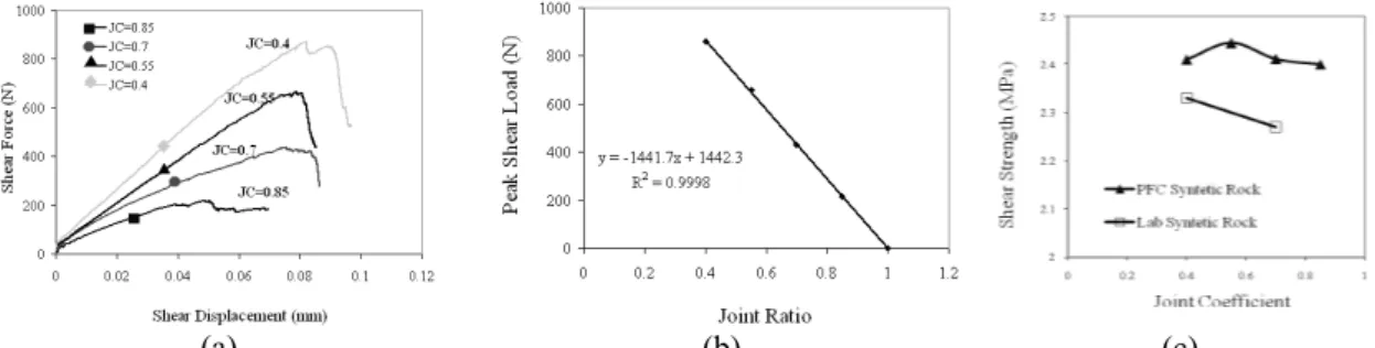
Fig. 16a illustrates the relationship between peak shear load and shear displacement and Fig. 16b represents the linear fitting curve of peak shear load and joint coefficient. Fig 16c show the variation of failure stress of bridged segment versus the joint coefficient for both of the numerical and physical models. The fill points and the hollow points represent the failure stresses in PFC2D models and laboratory samples; respectively. The failure stress is measured by division of maximum shear force to the Ligament length.
Through comparison between Figs. 12-15 and 16a, we can conclude that peak shear load is associated with the propagation length of the shear failure zone. The larger the propagation length is, the higher the peak shear load obtained.
From the linear fitting curve between peak shear load and joint coefficient shown in Fig. 16b, we can see that the peak shear load is almost linear to the joint coefficient. The smaller the ratio (JC=0.4) is, the higher the peak shear load is gained. Note that, increasing in loading capacity of rock bridge is not only due to increasing in the rock bridge length but also it can be explained by the Fracture Mechanics Theory, which indicates that for small joint lengths correspond small values of the Stress Intensity Factors (KI and KII). This leads to higher rock bridge strength. From the fitting equation, y = -1441.7x + 1442.3, as shown in Fig. 16b, it can be inferred that when specimen has no pre-existing joints, the joint coefficient is equal to 0, the peak shear load is 1442.3N. When the ideal condition that joint runs through the whole specimen (JC=1) occurs, the shear load is 0.6N, approximately close to 0. Therefore, the numerical results are in reasonable accordance with engineering reality.
(a) (b) (c)
Fig. 16. a) The relationship between peak shear load and shear displacement, b) The linear fitting curve of peak shear load and rock bridge ratio, c) The variation of failure stress of bridged segment versus the
From Fig 16c, it’s clear that the numerical simulation predicts shear strength of non-persistent joint approximately near to the experimental tests results. It’s clear that the capacity of bridged rock to resist shear loading has a close relationship with joint coefficient. With increasing the joint coefficient, the shear strength of rock bridged is reduced as a result of increasing in both of the stress concentration at tip of the joints and stress interaction between the joints.
From the above discussion, it can be concluded that the peak shear load of jointed rock is mostly influenced by failure pattern while the failure pattern of bridged rock is mainly controlled by the joint separation.
4.2. Echelon non-persistent joints 4.2.3. Failure pattern in the models:
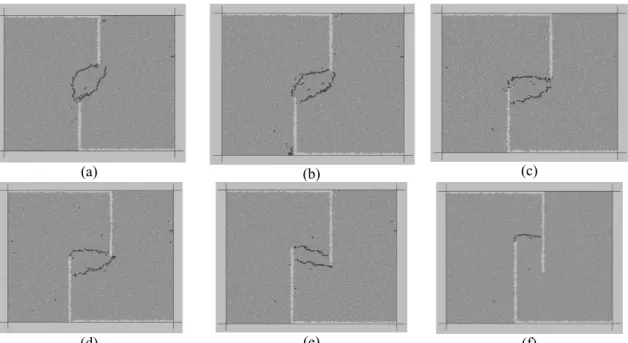
Fig. 17 displays the failure patterns in the samples. In these pictures, the black line and the red line represent the tensile crack and the shear crack, respectively.
(a) (b) (c)
(d) (e) (f)
Fig. 17. The failure patterns in the samples with different ligament angle, Ligament length=18mm, a) Ligament angle =25°, b) Ligament angle =50°, c) Ligament angle =75°, d) Ligament angle =90°, e)
Ligament angle =115°, f) Ligament angle =140°.
When ligament angles are 25° and 50°; the upper and lower wing cracks develop from the joint tips and
propagate out of the zone of maximum compressive force till coalesce with the opposite joint tip (fig 17 a and b). This coalesce left an elliptical. As can be seen from fig 5c, the same failure pattern has occurred in the physical samples when ligament angle is 25°.
When ligament angles are 75° and 90°; the upper wing crack develops from the tip of the upper joint while
the lower wing crack develops from the wall of the lower joint (fig 17 c and d). These wing cracks propagate through the intact portion area till coalesce with the opposite joint tip. As can be seen from fig 5d, nearly the same failure pattern has occurred in the physical samples when ligament angle is 90°.
When ligament angle is 115°; as seen in Fig. 17e, both of the upper and lower wing cracks develop from
the upper and lower joint walls; respectively. These wing cracks propagate through the intact portion area till coalesce with the opposite joint tips. As can be seen from fig 5e, the same failure pattern has occurred in the physical samples when ligament angle is 115°.
When ligament angle is 140°; as seen in Fig. 17f, only one wing crack develops from the wall of the upper
joint and propagates perpendicular with shear load direction till coalesces with the opposite joint tip. Fig 18 shows the ratio of tensile crack to shear crack number at three stage of the simulation for different joint configurations.
Ligament
angle to shear crack number (Ns) at different The ratio of tensile crack number (Nt) stages of the simulation (Nt/Ns)
A B C 25° 12/1 37/4 104/12 50° 11/1 39/1 127/2 75° 9/1 24/3 90/13 90° 7/1 64/3 95/4 115° 8/0 65/2 80/2 140° 3/0 24/1 33/1
Fig 18. The tensile crack to shear crack number ratio at each stage of the simulation for different ligament angle.
The crack ratio shown in Fig. 18 clearly reveals that, for each ligament angle, tension cracks are considerably greater in number than shear cracks at different stages of the simulation. Such differences are even more significant as shear displacement increases. It shows that the fracture morphology at low normal load level (0.33 MPa) did not result from shear stresses, but rather from tensile stresses.
When ligament angles are less than 90°, nearly 34% of total crack numbers develop at the peak strength
(stage B in solid line) and the final percent develop after the peak shear resistance is reached (stage C in solid line). It shows that the non-overlapped joint lost their loading capacity when 34% of total cracks develop within the rock bridge.
When ligament angles are more than 90°, only a few percent of total cracks less than 10% develop at the
peak strength (stage A in dotted line), and the final percent develop after the peak shear resistance is reached. It shows that the overlapped joint lost their loading capacity when cracks initiates at the joint tips.
4.2.5. Loading capacity of non-persistent joints
The relationship between the shear load and the shear displacement for each ligament angle is shown in Fig. 19.
Shear behavior of non-overlapped joint:
When ligament angles are less than 90° (non-overlapped joints); the load-displacement curves are
consisted of both of the linear and non-linear parts. It means that the models with non-overlapped joints have gone through yield deformation before its final failure. Such fracture is a progressive failure process. Note that, with increasing the ligament angle from 0° to 90°, the linearity part of force-displacement curve
is decreased and its non-linearity part is increased. The following reason can be accounted for this behavior:
When ligament angle is 0°, under the normal loading, only elastic deformation occurs in horizontal
direction while normal load has not any effect on the elastic behavior in shear direction. Therefore, the model shows large elastic deformation under the shear loading. With increasing the shear loading, the linear part changes to non-linear as a result of the crack initiation in bridged segment.
When ligament angles are more than 0°, under the normal loading, the bonded particles deform elastically
in both of the normal and shear direction due to orientation of ligament. In fact, the most part of linear behavior of model is mobilized under the normal loading, which is not registered, and the residual one is mobilized under the shear loading. As can be seen from fig 19, when ligament angles are 25°, 50° and 75°,
the force-displacement curve shows a small residual elastic deformation at the beginning of shear loading and then it shows a non-linear behavior as a result of plastic deformation.
Shear behavior of overlapped joint:
When ligament angles is more than 90° (overlapped joints); the load-displacement curve is completely
linear for overlapped joints (fig. 19). In fact, the models with overlapped joints have reached theirs peak shear load and got broken before they get into non-linear deformation stage. Such fracture is a brittle behavior process. In these configurations, the effect of normal load on the failure plane is eliminated completely because of the joint overlapping and only the tensile force is distributed in the bridged area. Whereas the bonded particles assembly has brittle behavior under tensile loading (resulted from the tensile stress-displacement curve in numerical Brazilian test (fig. 9)), therefore the shear force versus shear displacement curve is completely linear for overlapped joints as a result of pure tensile failure in the bridged segment.
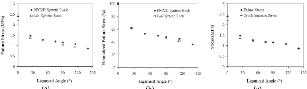
Fig 20a shows the variation of failure stress of bridged segment versus the ligament angle. Fig 20b shows the variation of normalized failure stress versus the ligament angle (the failure stresses in echelon joints have been normalized with failure stress in planar non-persistent joint). The fill points and the hollow points represent the failure stresses in PFC2D models and laboratory samples; respectively.
Fig 20c shows the crack initiation stress versus the ligament angle in PFC2D simulations. Also a comparison between the failure stress and crack initiation stress has been shown in this figure. The fill points and the black line represent the failure stresses and crack initiation stress; respectively.
(a) (b) (c)
Fig 20. a) The variation of failure stress of bridged segment versus the ligament angle; b) the variation of normalized failure stress versus the ligament angle; c) the crack initiation stress versus the ligament angle. From fig 20a, it’s clear that the numerical simulation predicts shear strength of non-persistent joint approximately near to the experimental tests results. It’s clear that the capacity of bridged rock to resist shear loading has a close relationship with ligament angle. The lower the ligament angle is, the higher the peak shear load obtained. It can be find from Figure 20a that the strength of overlapped joints, when ligament angle is more than 90°, is lower than the strength of non-overlapped joints. In fact, when
ligament angle is more than 90°, the effect of external normal load is eliminated on the bridged segment
and only tensile force chain resulted from external shear loading is distributed within the rock bridge as a result of joint overlapping. in other cases, when ligament angle is less than 90°, both of the tensile force
and compressive force chains are distributed within the rock bridge as a result of appearance of both of the external shear stress and normal stress on the rock bridge. Whereas the strength of bonded particles under the pure tensile loading is less than their strength under the mixed loading, therefore it can be concluded that the shear strength of overlapped joint is less than the shear strength of non-overlapped joint.
From above discussions it can be concluded that the ligament angle has significant effect on the shear strength of samples and also affected the initiation stress of the first crack. In fact, the peak shear load of jointed rock is mostly influenced by failure pattern while the failure pattern of bridged rock is mainly controlled by the joint overlapping. Whereas shear strength as one of material mechanical properties has a close relationship with its defect configuration, therefore the capacity of rock mass to resist shear loading is severely influenced by its macroscopic joint constellation i.e. joint separation and joint overlapping.
Conclusion:
The numerical study has demonstrated a more reasonable theoretical explanation for the shear mechanism of non-persistent joints due to the inner damages that are difficult to observe in an experimental testing. The shear behavior (failure progress, failure pattern, failure mechanism and shear strength) of rock like specimens containing two edge joints with different separation and overlapping has been investigated through of direct shear test using both of the PFC2D numerical simulation and experimental test. The whole shear failure process is visually represented and the failure pattern is obtained. The following
conclusions can be drawn from this research:
• With careful choice of intact rock micromechanical parameters, using a rigorous inverse modeling calibration procedure, it has been shown that PFC2D could be used in modeling the strength behavior of rock bridge under direct shear loading.
• In both of the planar and echelon non-persistent joint, the numerical simulations showed that dominant mode of fracturing, regardless of the stage of shearing, is tension.
• The numerical simulation on synthetic rock showed similar fracture patterns to those observed in the experimental test.
• Laboratory and numerical experiments presented in this paper show that there is a great dependence of failure pattern on the joint separation and joint overlapping. The failure patterns have also been shown to control the failure stress.
• In planar non-persistent joint, with increasing the joint coefficient the complex rupture surface changes to single symmetrical failure surface. In echelon non-persistent joint, the elliptical mode of coalescence changes to single failure surface with increasing the ligament angle.
• The shear strength of planar persistent joints is more than shear strength of echelon non-persistent joints. Also, Shear strength of echelon joints decrease as the ligament angle is increased.
• The planar non-persistent joint lost their loading capacity when 45% of total cracks develop within the rock bridge.
• The non-overlapped echelon joints lost their loading capacity when 34% of total cracks develop within the rock bridge while the overlapped echelon joint lost their loading capacity when 8% of total cracks develop within the rock bridge.
• The results from this work highlight the importance of tensile fracturing in the development of a shear zone at low normal stresses in non-persistent joint.
• Note that, the ratio of the minimum particle radius to the joint opening in PFC2D modeling was 0.27 that is too high in contrast with that in experimental test. If this ratio was reduced near to the physical one, the crack growth processes (such as initiation, propagation and coalescence) could be simulated in a high similarity with the natural condition. However, this takes a high code running time.
• Though the results presented in this paper are limited to blocks with open non-persistent joint sets under low normal load, experimental and numerical work on modeling rock bridge strength behavior under high normal load is currently in progress.
References
[1] Committee on Fracture Characterization and Fluid Flow, et al. Rock fractures and fluid flow. contemporary understanding and applications. Washington, DC: National Academic Press, 1996. [2] Einstein, H.H., D. Veneziano, G.B. Baecher and K.J. O’Reilly, 1983. The effect of discontinuity
persistence on rock slope stability. Intl. J. Rock Mech. Min. Sci. Geomech. Abstr.l 20 (5): 227-236. [3] Jaeger, J.C., 1971. Friction of rocks and stability of rock slopes. Geotechnique, 21: 97-134.
[4] Lajtai EZ. Strength of discontinuous rocks in direct shear. Geotechnique 1969;19:218_332. [5] Lajtai EZ. Shear strength of weakness planes in rock. Int J Rock Mech Min Sci 1969;6:499_515. [6] Savilahti T, Nordlund E, Stephansson O. Shear box testing and modeling of joint bridge. In:
Proceedings of international symposium on shear box testing and modeling of joint bridge Rock Joints, Norway, 1990. p. 295_300.
[7] Wong RHC, Leung WL, Wang SW. Shear strength study on rock-like models containing arrayed open joints. Rock mechanics in the national interest. In: Elsworth D, Tinucci JP, Heasley KA, editors. Swets & Zeitlinger Lisse, 2001. p. 843_9. ISBN:90-2651-827-7.
[8] Ghazvinian, A., M.R. Nikudel and V. Sarfarazi, 2007. Effect of rock bridge continuity and area on shear behavior of joints. 11th congress of the international society for rock mechanics, Lisbon,
Portugal.
[9] Gehle, C. and H.K. Kutter, 2003. Breakage and shear behavior of intermittent rock joints. Intl. J. Rock Mech. Min. Sci., 40: 687-700.
[10] Glynn EF, Veneziano D, Einstein HH. The probabilistic model for shearing resistance of jointed rock. In: Proceedings of the 19th US symposium on rock mechanics, Stateline, Nevada, 1978. p. 66-76. [11] Carpinteri A, Valente S. Size-scale transition from ductile to brittle failure: a dimensional analysis
approach, Proceedings of the CNRS-NSF, Workshop on strain localization and size effect due to cracking and damage, Cachan, 1988. p. 447-90.
[12] Blandford AR, Ingraea AR, Ligget JA. Two dimensional stress intensity factor computations using the boundary element method. Int J Num Method Eng 1981; 17: 387-401.
[13] Altiero NY, Gioda G. An integral equation approach to fracture propagation in rock. Riv Ital Geotecnica 1982; 387-404.
[14] Aliabadi MH, Brebbia CA. Advances in boundary element methods for fracture mechanics. Amsterdam: Computational Mechanics Publications, Elsevier, 1993.
[15] Vasarhelyi B, Bobet A. Modeling of crack initiation, propagation and coalescence in uniaxial compression. Rock Mech Rock Eng 2000; 33(2): 119-39.
[16] Erdogan F, Sih GC. On the crack extension path in plates under plane loading and transverse shear. ASMEJ Basic Eng 1963; 85: 516-27.
[17] Hussain MA, Pu EL, Underwood JH. Strain energy release rate for a crack under combined model I and mode II. ASTM STP 1974; 560: 2-28.
[18] Sih GC. Strain-energy-density factor applied to mixed mode crack problems. Int J Fract 1974; 10: 305-21.
[19] Reyes O, Einstein HH. Failure mechanism of fractured rock- a fracture coalescence model. Proceeding of the Seventh Congress of the ISRM, vol. I, 1991; p. 333-40.
[20] Shen B, Stephansson O. Modification of the g-criterion for crack propagation subjected to compression. Eng Fract Mech 1994; 47(2): 177-89.
[21] Bobet A, Einstein HH. Numerical modeling of fracture coalescence in rock materials. Int J Fracture 1998; 92: 221-52.
[22] Scavia C, Castelli M. In: Barla G, editor. Analysis of the propagation of natural discontinuities in rock bridges, EUROCK’98. Rotterdam: Balkema, 1996. p. 445-51.
[23] Scavia C. The displacement discontinuity method for the analysis of rock structures: a fracture mechanic. In: Aliabadi MH, editor. Fracture of Rock. Boston: WIT press, Computational Mechanics Publications, 1999. p. 39-82.
[24] Bobet, A. and H.H. Einstein, 1998. Fracture coalescence in rock-type materials under uniaxial and biaxial compression. Intl. J. Rock Mech. Min. Sci., 35: 863-888.
[25] PFC2D (Particle Flow Code in 2 Dimensions). Version 3.1. Minneapolis: Itasca Consulting Group; 1999.
[26] Potyondy DO, Cundall PA. A bonded-particle model for rock. Int J Rock Mech Min Sci 2004; 41: 1329-64.
[27] Cho N, Martin CD, Sego DC. A clumped particle model for rock. Int J Rock Mech Min Sci 2008; 45: 1335-1346.
[28] Wong RHC, Chau KT, Tsoi PM, Tang CA. Pattern of coalescence of rock bridge between two joints under shear testing. In: Vouile G, Berest P, editors. The 9th international congress on rock mechanics, Paris, 1999. p. 735-8.