Linking entanglement detection and state tomography via quantum 2-designs

PAPER • OPEN ACCESS

Linking entanglement detection and state tomography via quantum

2-designs

To cite this article: Joonwoo Bae et al 2019 New J. Phys. 21 013012

View the article online for updates and enhancements.

PAPER

Linking entanglement detection and state tomography via quantum

2-designs

Joonwoo Bae1,2

, Beatrix C Hiesmayr3,6

and Daniel McNulty4,5

1 _{School of Electrical Engineering, Korea Advanced Institute of Science and Technology(KAIST), 291 Daehak-ro, Yuseong-gu, Daejeon}

34141, Republic of Korea

2 _{Freiburg Institute for Advanced Studies(FRIAS), Albert-Ludwigs University of Freiburg, Albertstrasse 19, D-79104 Freiburg, Germany} 3 _{University of Vienna, Faculty of Physics, Boltzmanngasse 5, A-1090 Vienna, Austria}

4 _{Department of Mathematics, Aberystwyth University, Aberystwyth, United Kingdom} 5 _{Faculty of Informatics, Masaryk University, Brno, Czechia}

6 _{Author to whom any correspondence should be addressed.}

E-mail:Beatrix.Hiesmayr@unvie.ac.at

Keywords: mutually unbiased bases, symmetric informationally complete POVM, entanglement detection

Abstract

We present an experimentally feasible and efficient method for detecting entangled states with

measurements that extend naturally to a tomographically complete set. Our detection criterion for

bipartite systems with equal dimensions is based on measurements from subsets of a quantum

2-design, e.g. mutually unbiased bases or symmetric informationally complete states, and has several

advantages over standard entanglement witnesses. First, as more detectors in the measurement are

applied, there is a higher chance of witnessing a larger set of entangled states, in such a way that the

measurement setting converges to a complete setup for quantum state tomography. Secondly, our

method is twice as effective as standard witnesses in the sense that both upper and lower bounds can be

derived. Thirdly, the scheme can be readily applied to measurement-device-independent scenarios.

executes, which utilizes an entanglement witness that works with individual measurements followed be post-processing of the outcomes[3], to provide an experimentally feasible approach for this task [4]. Entanglement

detection under less assumptions, for instance, when detectors are not trusted[5–7] or dimensions are unknown

[8], is of practical significance for cryptographic applications.

For the practical usefulness of entanglement detection, it is worth exploring the experimental resources. If a priori information about a quantum state is given, a set of entanglement witnesses may be constructed accordingly and exploited for entanglement detection. With no a priori information multiple entanglement witnesses may be required. One possible method is quantum state tomography which determines a d-dimensional quantum state with O(d2_{) measurements. Then, theoretical tools such as positive maps [}

9], e.g.

partial transpose, or numerical tests involving semidefinite programming [10] can be applied. For entanglement

witnesses, however, little is known about the minimal measurements for their realization. In fact, it may happen that repeating experiments for multiple witnesses may be less cost effective than state tomography[11], and

quite possible that no useful information is obtained, neither for entanglement detection nor for quantum state identification. This raises questions on the usefulness of entanglement witnesses, in particular when a priori information about a particular state is not available.

A useful experimental setup for entanglement detection may distinguish the largest collection of entangled states with as few measurements as possible. It is noteworthy that a tomographically complete measurement can ultimately identify a quantum state so that theoretical tools may completely determine whether it is entangled or separable. From a practical point of view, it would be therefore highly desirable that measurements for entanglement detection are constructive, i.e. they can be extended to a tomographically complete set by augmenting more detectors.

In this work we establish a feasible and practical framework of entanglement detection by applying a subset of measurements taken from a quantum 2-design, namely mutually unbiased bases(MUBs) [12] and a OPEN ACCESS

RECEIVED

15 August 2018

REVISED

9 November 2018

ACCEPTED FOR PUBLICATION

14 December 2018

PUBLISHED

18 January 2019

Original content from this work may be used under the terms of theCreative Commons Attribution 3.0 licence.

Any further distribution of this work must maintain attribution to the author(s) and the title of the work, journal citation and DOI.

symmetric informationally complete(SIC) positive-operator-valued-measure (POVM) [13]. The connections

between entanglement detection, MUBs, and quantum 2-designs havefirst been explored in [14,15], and

subsequent results were found in, e.g.[16–18]. Let us emphasize here that entanglement detection via MUBs can

also detect bound entangled states, those mixed entangled states from which no entanglement can be distilled. Furthermore, measurement setups with MUBs are very experimentally friendly, indeed the MUB criterion[14]

resulted in thefirst experimental demonstration of bipartite bound entanglement [19], predicted in 1998 [20].

Here we present a unifying approach to these connections with a three-fold advantage. First, by using incomplete sets of MUBs and subsets of a SIC-POVM, the entanglement detection scheme then extends naturally to an optimal reconstruction of the quantum state[21,22]: once direct detection of entanglement fails,

additional detectors are applied in the measurement scheme to distinguish a larger set of entangled states, and can be ultimately utilised tofind its separability via state tomography. This demonstrates in a natural framework that larger sets of detectors are more useful for distinguishing entangled states. Next, our results have twice the efficiency of standard witnesses, in the sense that both a lower and upper bound for separable states exist, whereas entanglement witnesses have only the zero-valued lower bound. Finally, the scheme can be readily applied to a measurement-device-independent(MDI) scenario for which the assumptions on the detectors are relaxed. This can be achieved by converting the measurement into the preparation of a quantum 2-design.

Let us begin with a brief summary on the implementation of entanglement witnesses in practice.

Entanglement witnesses correspond to observables that have non-negative expectation values for all separable states as well as negative values for some entangled states. They can be factorized into local observables in general, which are then decomposed by POVM elements[23]. A witness W can be written with POVMs denoted

by M_{{ i}( )X_{}for party X=A, B, where the measurement is complete, i.e. M I}

i iX X

å

Xdenotes the

identity operator on system X, as

W c M, where M M M , 1

i

i i i iA iB

å

= = ( )Ä ( ) ( )

with constants{ }ci . In implementation, a POVM can be realized by projective measurements with ancillary

systems, see e.g.[24]. For a state ρ, the probabilitiesPr[Mi∣ ]r =tr[rMi]are estimated experimentally by the

detectors M{ i}. Then, the expectation value of W for a stateρ is obtained by computing the linear combination,

c PrM

i i i

å

Although the factorization with local measurements in equation(1) is not necessary to realize entanglement

witnesses, it provides a natural framework for converting standard entanglement witnesses to the MDI scenario that closes all loopholes arising from detectors. In such a scenario two parties Alice and Bob, who want to learn if an unknown quantum stateρABis entangled, prepare a set of quantum states, after which a measurement is

performed by untrusted parties. A standard witness in equation(1) can be used to construct an MDI

entanglement witness as follows

W c M M , 2

i

i iA iB

MDI=

å

where the transposeis performed in a chosen basis of for YY =A B, [6]. The separable decomposition in

equation(2) shows which quantum states the two parties must prepare,{M~_i( )A}and{M~_i( )B}, where

M_iY =M_iY tr M_iY

~

[ ]

( ) _{( ) ( )}

/ correspond to the quantum states.

Let us reiterate that entanglement witnesses with local measurements in equation(1) are readily converted to

their counterparts in an MDI scenario, where entangled states are detected with less assumptions. We also note that, to the best of our knowledge, there is no general and systematic way offinding the factorization with a minimal number of local measurements. The decomposition with a minimal number of POVM elements is essential, as mentioned, to take advantage of entanglement witnesses that can detect entangled states without state tomography.

We now introduce particular sets of POVMs called quantum 2-designs. A set of quantum states{∣y ñi}kin a

d-dimensional Hilbert space,∣y ñ Îi d, or their corresponding rank-one projectors, is called a quantum

2-design if the average value of any second order polynomial over the set{∣y ñi }kis equal to the average f y( )over

all normalized states∣yñ, for the Haar measure. This holds true if and only if the average of∣y yiñá i∣Ä2over the

entire 2-design is proportional to the symmetric projection ontodÄd. Examples of quantum 2-designs

include a complete set of d( +1)MUBs, and a SIC-POVM containing d2elements, which are defined as follows. Let =k {∣bikñ}di=1denote an orthonormal basis in the Hilbert spaced. A set of m bases{k k}m=1are

mutually unbiased if b b d 1 1 , 3 ik ik 2 dkk d dii kk á ¢¢ñ = - ¢ + ¢ ¢ ∣ ∣ ∣ ( ) ( )

for i i, ¢ = ¼ , and k k1, ,d , ¢ = ¼1, ,m. Let Sd sj dj 1

2

={∣ ñ}₌ denote a set of d2vectors in the same Hilbert space

d

s s d d 1 1 , 4 j j jj 2 d á ñ = + + ¢ ¢ ∣ ∣ ∣ ( ) ( ) for all j j, _{¢ = ¼}1, ,d2_.

The existence of d( +1)MUBs and d2SIC states in all dimensions have been long-standing open problems in quantum information theory[25]. For instance, complete sets of MUBs are known to exist in prime-power

dimensions[21,26–29] but have not been found in in any other composite dimension. For example, when

d=6, it is conjectured that only 3 MUBs exist [30,31], but no proof exists. While it is conjectured that a

SIC-POVM exists for any d, the largest dimension for which an exact solution has been found is d=323 [32].

It is well known that a full set of d( +1)MUBs and a SIC-POVM are tomographically complete:

measurements from either set determine a quantum state uniquely. Furthermore, the sets are both optimal and simple for quantum state tomography, in that they minimize the error of the estimated statistics while at the same time having exceptionally simple state reconstruction formulas[21,22]. Note that both MUBs and

SIC-POVMs are experimentally feasible, and have been implemented for the purpose of state tomography. A recent demonstration has been given in[33].

We now consider subsets of d( +1)MUBs and d2SIC vectors for detecting entangled states. We denote by

I_{m d}( )M_{, andI} m d,

S

~( ) the collections of probabilities when the measurements are applied in MUBs and SICs, respectively,

I_{m d} : _{k k}m Pr ,i i , , 5 k m i d k k , M 1 1 1 

å å

å

whereSm~denotes a collection ofm~states out of d2SIC vectors, andPr(a b, ∣A B, )the probability of

obtaining outcome(a b, )given a measurement in A and B. To be explicit, for stateρ,Pr ,(i i∣  =k, k)

b b b b

tr[∣ _ikñá _ik∣ ∣Ä _ikñá _ik∣ ]r7andPr ,(j j S∣ m~,Sm~)=tr[∣sjñá Ä ñásj∣ ∣sj sj∣ ]. These probabilities can be obtainedr

simply by preparing local measurements in MUBs or SICs. Note that we have m + and md 1 ~d2_,

where the equality corresponds to cases in which the measurement setting is tomographically complete. Since the set of all separable states forms a convex set, the quantities I_{m d}( )M_{, andI}

m dS,

~( ) as defined in equations (5)

and(6) have both nontrivial upper and lower bounds satisfied by all separable states. In what follows, the bounds

for selections of m MUBs andm~SIC vectors are explicitly presented. We minimize and maximize each of the bounds with respect to the set of MUBs and SIC vectors, e.g. minimizing(maximizing) the lower bound over all MUBs gives L_{m d}-( )_,M (L_{m d}+( )_,M). The former (latter) gives a bound which is independent (dependent) of the choice of MUBs. Consequently, L_{m d}+( )_,M detects a larger set of entangled states but only applies for a certain collection of MUBs.

When the measurements are taken from a set of MUBs, the minimal and maximal lower bounds, L_{m d}-( )_,M and

L_{m d}+( )_,M, respectively, are given by

L_{m d}, min min I_{m d} : k km , 7 M , M sep 1 k k m 1 sep   s = s -= = ( { } ) ( ) ( ) { } ( )

L_{m d,}M max k k min I_{m d}M_, sep: _{k k}m 1 , 8

m 1 sep   s = s + = = ( { } ) ( ) ( ) { } ( )

where the optimisation is taken over all separable statess and all possible collections of m MUBs,sep {k k}m=1, that

exist in dimension d. It is clear that L_{m d}+_,( )M L_{m d}-_,( )M_{, and the gap between the bounds is due to different sets of m}

MUBs having different overlaps with the set of separable states.

Unfortunately, we do notfind a systematic and general method of obtaining these bounds but had to consider all possible sets of m MUBs, minimizing I_{m d}( )M_, over all separable states. In table1, lower bounds are shown for d=2, 3, 4, which are obtained analytically. It turns out that L_{m d}-_,( )M =L_{m d}+_,( )M _{for d=2, 3, but for}

d=4 we found Lm-,4( )M Lm+,4( )M. The difference here is due to the existence of an infinite family of 3 MUBs in

d=4, resulting in unitarily inequivalent triples. The triple which gives L_m,4-( )M =1 4is the only extendible set of 3 MUBs, in the sense that no other triple extends to a complete set of 5 MUBs. For d=2, 3,all subsets of m MUBs are equivalent and extendible.

In[14], it has been shown that the upper bound does not depend on selections of MUBs, and is given by

U I m d max : 1 1, 9 m d, m d k km M , M sep 1 sep s  = s ( { }= )= + - ( ) ( ) ( )

for any m MUBs{k k}m=1. Note that in the case of a quantum 2-design with m=d+ , the upper bound1

satisfies U_d( )M_+1,d =2_{, which is independent of the dimension d. Notice also that by removing a single basis from}

7

Note that Alice and Bob may consider an unphysical relabelling of their basis vectors in order to optimize the correlation function. In particular, for the isotropic state a complex conjugation in one subsystem gives the optimum.

I_{m d}( )M_{, the upper bound decreased uniformly by1 d, i.e.}

U_mM_1,d-U_{m d}M_{, =} d 1

+

-( ) ( )

for all mMUBs.

In ourfirst main result, using table1and equation(9), we can construct the inequalities with optimization

over m MUBs in equation(5) as

L_{m d}-_,( )M I_{m d}( )M_, (ssep)U_{m d}( )M_, , (10) that are satisfied by all separable states indÄd. A quantum state must be entangled if it violates one of the

inequalities above, see alsofigure1. It is also worth mentioning that these inequalities detect bound entangled states when m=d+ , as shown in1 [19].

In a similar way, lower and upper bounds for SICs are denoted as follows, with g = , and opt+=maxand opt-=min,

L_{m d}g_,S optg_{Sm S} min I_{m d}S_, sep:Sm and 11

d2 sep s = _Í s ~( ) _~ ~( )₍ ~_{) ( )} U_{m d}g, opt_Sg _S max I_{m d} :Sm , 12 S , S sep m d2 sep s = _Í s ~( ) _~ ~( )( ~) ( )

whereSm~is a set ofm~SIC vectors. Then, the full set of SIC vectors is denoted by Sd2. Again, we do notfind a

systematic and general method of computing upper and lower bounds. However, having explored all possible subsets of SIC vectors in d=2, 3, for a given SIC-POVM, we present these bounds in table2. Suboptimal bounds for d=4 are also presented in the appendix. We observe that U_{m d,}S U_{m d}

,S



+

-~( ) ~( ), i.e. differences in the subsets of SIC vectors give rise to the gap between these upper bounds. Therefore, the inequalities which are satisfied by all separable states are constructed in our second main result as

L_{m d,}S I_{m d}S_, sep U_{m d}, , 13

S

 s 

- +

~( ) ~( )( ) ~( ) ( )

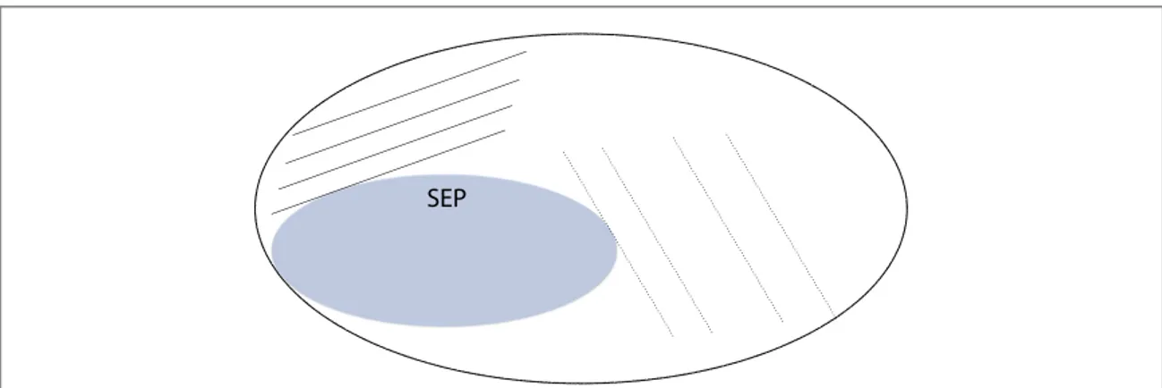
Figure 1. Our strategy for detecting entangled states via MUBs and SICs is illustrated, where X=M, Sandn=m m,~, see inequalities in equations(10) and (13) satisfied by all separable states. Violation of the bounds implies detection of entangled states.

Once the measurement outcomes are collected, they are exploited twice tofind if the upper or lower bound is violated, in which case entangled states are detected.

Table 1. Lower and upper bounds on MUBs, L_{m d}( )_,M _andU

m d, M

( )_{, see equations(7)–(9), are}

summarized for m MUBs in_=d_{, ford=2, 3, 4. For d=2, 3, inequivalent sets of m}

MUBs do not exist, hence we haveL_{m d,}M L_{m d} ,M

=

+( ) -( )_{. This is no longer true for d=4, as seen}

when m=3.

Lower bounds Upper bounds

d=2 d=3 d_=4 d=2 d=3 d=4 m Lm,2( )M Lm,3( )M Lm,4-( )M Lm,4+( )M Um,2( )M Um,3( )M Um,4( )M 2 1/2 0.211 0 0 3/2 4/3 5/4 3 1 1/2 1/4 1/2 2 5/3 6/4 4 1 1_/2 1_/2 2 7_/4 5 1 1 2

where L_{m d~}-_,( )S _andU m d,S

+

~( )are found in table2. Even tighter inequalities withL_{m d~}+_,( )S _{and U} m d,S

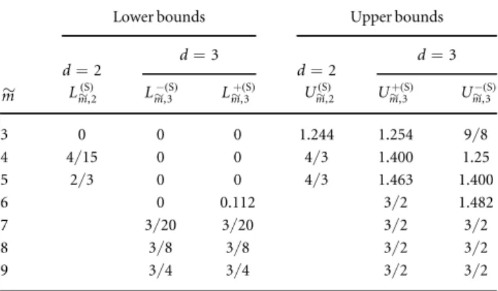
-~( )can be derived by specifying the corresponding subset ofm~SIC vectors. We note that for largem~the upper bounds become independent of the choice of SIC vectors, e.g. U_m~+_,3( )S =U_m~-_,3( )S =3 2for m~=7, 8, 9.

While these inequalities have been obtained by extensively considering all sets of MUBs and SIC vectors, analytic expressions for the upper and lower bounds can be derived for a quantum 2-design

I d d I d d 1 2, 1 2 1, 14 d 1,d d d M sep S2_, sep  s   s  + + + ( ) ( ) ( ) ( ) ( )

as shown in the appendix. The upper bounds to I_d( )M_{+1,dand I} d d,

S

2

( ) _{are proven in[14] and [17], respectively. Lower}

bounds are shown in[15] and later in [18]. As mentioned earlier, when the full measurement set of a quantum

2-design is used, it is more efficient to exploit the measurements for state tomography, and use theoretical tools to solve the separability problem that is known to be NP-hard.

To illustrate the effectiveness of the inequalities in equations(10) and (13), consider the isotropic and

Werner states,

p p p

Werner state: r_W = Psym+ 1- Pasym 15

~ ~

( ) ( ) ( )

q q q

isotropic state: riso( )= F ñáF +∣ + +∣ (1- )dÄd, (16) wherePsym

~

andPasym ~

denote the normalized projections onto the symmetric and anti-symmetric subspaces, respectively, andd = d, the normalized identity operator in dimension d. We note that for a bipartite Hilbert

spaced_Äd_{, the symmetric subspace is the subspace of all vectors in}d_Äd_{which are symmetric under}

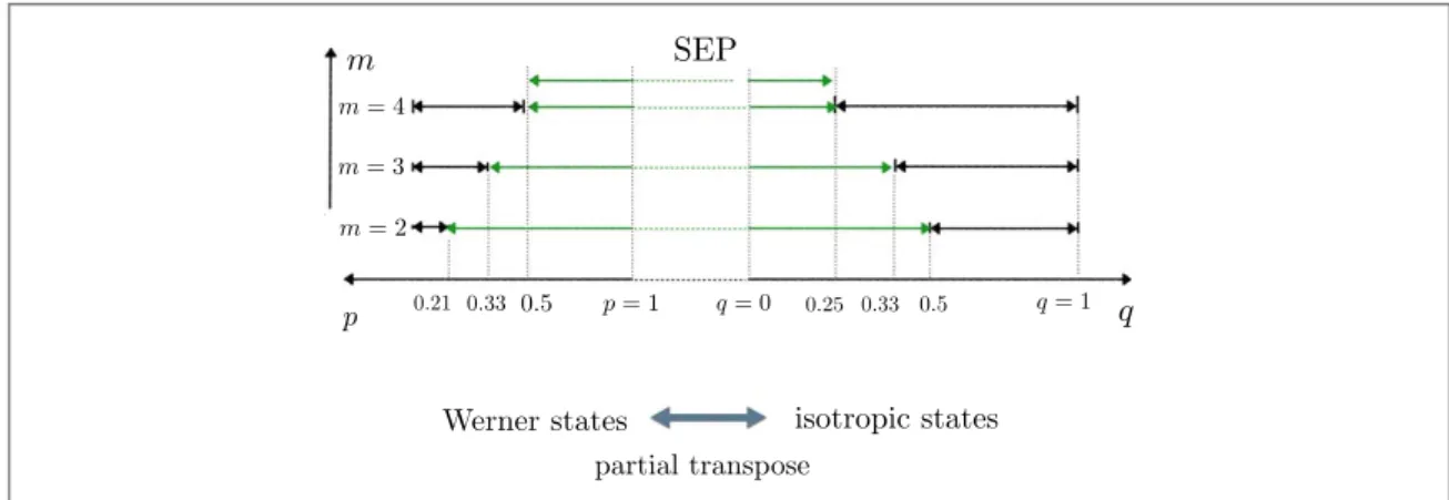
the interchange of their subsystems, while the anti-symmetric subspace is the subspace of all vectors that are negated by a permutation of their subsystems. It is known thatr_Wis entangled iff p <1 2andr_isoiff

q_>(d₊1₎-1_{. Infigure2, the capability of entanglement detection with I}

m,3( )M is shown for m=2, 3, 4. The

capability of entanglement detection via SICs is given in the appendix.

Due to the linearity of equations(5) and (6), with respect to the state ρ, one may expect that the inequalities in

equation(14) are closely connected to standard entanglement witnesses. Here we point out the equivalence

between the lower bounds in equation(14) and the partial transpose criterion, by considering the so-called

structural physical approximation[1]. For recent reviews on this see [2], as well as the appendix for further

details. The Choi–Jamiolkowski operator for the transpose map corresponds to an entanglement witness, denoted by W, i.e.tr[ssepW]0, andtr[rW]<0for some entangled statesρ which include the entangled Werner states in equation(15). By applying the structural physical approximation to the transpose map, the

resulting Choi–Jamiolkowski operator denoted by W~is given by W = Psym

~ ~

. The conditiontr[ssepW]0 then translates totrssepW  d d+1 1

~

-[ ] [ ( )] , see[15], which is equivalent to the lower bounds in equation (14).

Finally, we can see that I_{m d}( )M_, ( )r =tr[W_{m d}( )M_, r]and I_{m d}~( )S_, ( )r =tr[W_{m d}~( )S_, r]are readily converted for entanglement detection in a MDI scenario where,

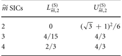
Table 2. The lower and upper bounds via SICs,L_{m d}_,S

~( )andU_{m d~}_,( )S_{, are shown}

for d_{=2, 3. We use the SIC-POVM defined in equations (}B.28_{) for d=2}

and the Hesse SIC defined in equations (B.32) for d=3. Note that L_m,2S L_m ,2 S = + -~( ) ~( )andU_m,2S U_m ,2 S = + -~( ) ~( ). In contrast to MUBs, we_find thatU_{m d}+~_,( )S U-_{m d}~( )_,S.

Lower bounds Upper bounds

d=2 d=3 d=2 d=3 m~ L_m,2~( )S L_m,3-~( )S L_m,3~+( )S U_m,2~( )S U_m,3~+( )S U_m,3~-( )S 3 0 0 0 1.244 1.254 9_/8 4 4/15 0 0 4/3 1.400 1.25 5 2/3 0 0 4/3 1.463 1.400 6 0 0.112 3/2 1.482 7 3/20 3/20 3/2 3/2 8 3/8 3/8 3/2 3/2 9 3/4 3/4 3/2 3/2

W b b b b W S s s s s , . m d k k m k m i d ik ik ik ik m d m j m j j j j , M 1 1 1 , S 1 

å å

å

As described in equation(2), both I_{m d}( )M_{, andI} m d,

S

~( ) can be obtained in an MDI manner with W_{m d}M_,  _{k k}m ₁

=

({ } )

( ) _and

W_{m d}, Sm S 

~( ) ₍ ~_{), respectively, by preparing the set of quantum states} k km 1

 =

{ } andSm~instead of measurements in

these bases. Note also that this provides both upper and lower MDI bounds as opposed to standard MDI entanglement witnesses.

To conclude, let us recall the problem addressed at the outset. How do we learn efficiently if an unknown quantum state is entangled, with a measurement that is tomographically incomplete? In this paper we propose a measurement setup for this purpose, which detects entangled states with cost effective measurements, and which extends naturally to a tomographically complete measurement for quantum state reconstruction. This latter feature is highly advantageous since it allows experimentalists to perform direct detection of entanglement with only a few measurements, and then, if necessary, to perform quantum state tomography by adding

additional measurements and using previous data. Thus, our scheme circumvents the highly non-trivial problem of comparing and connecting standard entanglement witness measurements with those which are useful for state tomography.

Our results also provide other advantages such as offering double the efficiency of standard and nonlinear witnesses, with both upper and lower bounds. One consequence of our analysis is that certain sets of MUBs are more‘useful’ for entanglement detection than others. For instance, in dimension d=4, the set of 3 MUBs which extends to a complete set provides the minimal(weakest) lower bound and therefore detects a smaller set of entangled states than unextendible MUBs. Thus, one might expect that unextendible MUBs are more useful in other dimensions too. We also note that the results can be generalized to weighted 2-designs[34], which

would allow for entanglement detection and state tomography in dimensions where the existence of MUBs and SICs is not yet known.

We envisage directions in entanglement detection beyond standard witnesses and towards related problems in quantum information theory. While we have already shown some links between standard entanglement witnesses and the MUB-inequality(10) and the SIC-inequality(13), we expect further connections to also hold

true. For example, recently it has been shown that MUBs can be used to construct positive but not completely positive maps, which lead to a class of entanglement witnesses[35]. Further relations in this direction may reveal

additional capabilities of entanglement witnesses at an even deeper level. It would also be interesting to consider nonlinearity, e.g. in[36], to improve the inequalities. We also hope that the presented framework of

entanglement detection may offer insightful hints towards a solution of the existence problem for MUBs and SICs from an entanglement perspective[25]. In addition, MUBs and SICs have quite recently been generalized

by relaxing the rank-1 condition to so-called mutually unbiased measurements and SIC measurements, which exist in allfinite dimensions [37]. Both of these, as well as other similar measurements, could be applied to our

framework in similar ways, leading to more experimentally feasible entanglement detection methods in arbitrary dimensions.

Figure 2. The inequalities I2,3( )M, I3,3( )M, and I4,3( )Mare applied to detect entangled states. OnceIm d, ( )M for unknown quantum states is

obtained, it can be utilized twice for entanglement detection with both upper and lower bounds. E.g. the upper bounds are violated by entangled isotropic states and the lower bounds by entangled Werner states.

Acknowledgments

JB is supported by the ITRC(Information Technology Research Center) support program (IITP-2018-2018-0-01402), the Institute for Information & communications Technology Promotion (IITP) grant funded by the Korea government(MSIP) (R0190-17-2028), National Research Foundation of Korea (NRF-2017R1E1A1A03069961), the KIST Institutional Program(2E26680-17-P025), and the People Programme (Marie Curie Actions) of the European Union Seventh Framework Programme(FP7/2007-2013) under REA grant agreement N 609305. BCH gratefully acknowledges the Austrian Science Fund FWF-P26783. DM has received funding from the European Union’s Horizon 2020 research and innovation programme under the Marie Skłodowska-Curie grant agreement No 663830. The authors are grateful to an anonymous referee for helpful comments.

Appendix A. Quantum 2-Designs, MUBs and SICs

In these appendices we review known results on quantum 2-designs, MUBs, SIC-POVMs, and entanglement witnesses. The main results are presented, including a derivation of the lower and upper bounds for inequalities which detect entangled states via collections of MUBs and SIC vectors. We analyse the capability of our criterion, and show that as we apply more measurements, i.e. as the number of MUBs and SIC vectors increase, the criterion detects larger sets of entangled states. When we apply a quantum 2-design, i.e. a full set of d( +1) MUBs or d2SIC vectors, the inequalities provide a necessary and sufficient condition for the separability of a certain class of quantum states, namely the symmetric states. We also show for quantum 2-designs how our detection criterion is related to entanglement witnesses.

Let us begin with a discussion on quantum 2-designs, also known as complex projective 2-designs, and recall two well known examples, a complete set of d( +1)MUBs and a SIC-POVM consisting of d2elements. An ensemble of n normalized d-dimensional vectors={∣ykñ Í} dis a quantum 2-design if the average value

of any second order polynomialf y( )over the set  is identical to the average of f y( )over the unitarily invariant Haar distribution of unit vectors_{∣yñ Î}d_{. To be precise,f y( )is a homogenous polynomial of degree}

two in the coefficients of∣yñand of degree two in the complex conjugates of these coefficients. In other words,  is a quantum 2-design if it has thefirst two moments equal to those of the Haar distribution. It can be shown that such an ensemble of vectors is a quantum 2-design if and only if

n d d 1 2 1 , A.1 i n i i 1 2 sym

å

wherePsymis the projector onto the symmetric subspace ofdÄd.

We write the symmetric and anti-symmetric projectors, 1 2 , and 1 2 d d d d sym   asym   P = ( Ä + P) P = ( Ä - P)

respectively, where denotes the identity operator in d-dimensional Hilbert space, and P corresponds to thed

permutation operator in_{ (} d_Äd_{). Note the useful relation thatP = F ñáF}G _d∣ + +_{∣, withΓ the partial}

transpose and ii d i d 1 1 F ñ =+ å ñ =

∣ ∣ the maximally entangled state.

Well known examples of quantum 2-designs are complete sets of d( +1)MUBs and SIC-POVMs. Let

b

k ik id 1

 ={∣ ñ}= denote an orthonormal basis of the space .d  andk k¢are called mutually unbiased if it holds

that for all i i, ¢, b b_{á i}k _ik_{ñ =}2 d 1

¢¢

-∣ ∣ ∣ . SIC states are a set of normalized vectors sjñmj=1 ~

{∣ } in_{ satisfying the relation}d

s sj j 2 d 1 1

á ¢ñ = +

-∣ ∣ ∣ ( ) for all j¹ ¢. The SIC states form a SIC-POVM when mj ~₌d2_{. Suppose that for a}

d-dimensional Hilbert space, there exist d( +1)MUBs and d2SIC states. Then, it holds that

d d b b d s s 1 1 1 , k d i d ik ik j d j j sym 1 1 1 2 2 1 2 2

å å

å

denotes the normalized projection onto the symmetric subspace,Psym=2 d d+1 1Psym

~

-[ ( )] .

Note that the existence of a complete set of MUBs and a SIC-POVM has been a long-standing open problem in quantum information theory and is related to several other unsolved problems in mathematics such as orthogonal decompositions of Lie algebras. It is conjectured that there exist d( +1)MUBs if and only if the dimension d is a prime-power, while a set of d2SIC vectors is conjectured to exist for all d[38]. So far, it is known

that complete sets of MUBs exist in all prime-power dimensions[21,26–29], while only significantly smaller sets

have been found in other composite dimensions. In particular, for dimension d=6, numerical calculations suggest that there exist only 3 MUBs[30]. On the other hand, numerical solutions of SIC-POVMs have been

Appendix B. Detecting entangled states using MUBs and SICs

Let us now consider incomplete sets of MUBs and subsets of a SIC-POVM for entanglement detection. We will formulate the inequalities in terms of probabilities, having both upper and lower bounds, which are satisfied by all separable states. Since the structure of MUBs and SICs is not fully understood, it is a non-trivial task to derive these bounds. For instance, in certain dimensions d, different equivalence classes of MUBs exist, and the bounds can often depend on the choice of a particular class. Furthermore, the bounds do not appear to have a simple analytical expression, behaving differently as the dimension changes. In the following, we willfirst consider entanglement detection with measurements corresponding to MUBs, and then apply similar techniques to derive bounds for SICs. Finally, we show the relationship between quantum 2-designs and entanglement witnesses.

We denote by I_{m d}( )M_{, andI} m d~S,

( )_{, collections of probabilities when measurements are applied from sets of MUBs}

and SIC vectors, respectively. For measurements of a set of m MUBs,{k k}m=1in , or a set Sd m~ Ídofm~SIC

states from a SIC-POVM, applied to each subsystem of a d( ´d)bipartite stateρ, these quantities are defined as,

I_{m d} : k km Pr ,i i , , B.1 k m i d k k , M 1 1 1 

å å

å

where we havePr ,(i i∣ k, k)=tr[∣bikñábik∣ ∣Äbikñábik∣ ]r andPr ,(j j S∣ m~,S~m)=tr[∣sjñá Ä ñásj∣ ∣sj sj∣ ]. We nowr

derive upper and lower bounds for the quantities I_{m d}( )M_, andI_{m d}~( )S_, , which hold true for all separable states. B.1. Lower and upper bounds of I_{m d}( )M_,

Let L_{m d}( )M_{, and U} m d,

M

( )_{denote the upper and lower bounds of I} m d,

M

( )_{, respectively, for a set of m MUBs,} k km 1

 =

{ } , with

m d

1<  + . We calculate these quantities by minimizing and maximizing over all separable states such that1

L_{m d} k km min Im d : k k , B.3 m , M 1 , M sep 1 sep  = = s s  = ({ } ) ( { } ) ( ) ( ) ( )

U_{m d}M_, ({_{k k}}m=₁)=maxssepI_{m d}M_, (ssep:{_{k k}}m=1). (B.4)

( ) ( )

For certain dimensions d, there exists inequivalent sets of m MUBs, up to unitary transformations. For instance, some sets extend to d( +1)MUBs while others are unextendible[41]. Thus, the bounds above may also have a

dependence on the choice of MUBs, and hence we also classify these additional bounds as follows

L_{m d,}M min _{k k}m L_{m d}M_{, k k}m ₁ , B.5 1   = -= = ({ } ) ( ) ( ) { } ( ) L_{m d,}M max _{k k}m L_{m d}M_{, k k}m ₁ , B.6 1   = + = = ({ } ) ( ) ( ) { } ( ) U_{m d},M min k k U_{m d}M, k km 1 , B.7 m 1   = -= = ({ } ) ( ) ( ) { } ( ) U_{m d},M =maxk km1U_{m d}M, k km 1 , B.8 + = = ({ } ) ( ) ( ) { } ( )

where the minimum and maximum are taken over all possible collections of m MUBs,{k k}m=1, that exist in

dimension d. Note that for d , all sets of MUBs are known [5 42,43]. However, for d , the complete6 classification of MUBs remains an open problem, even for prime-power dimensions, hence such an optimization is currently not possible in large dimensions.

It then follows we have the bounds

L_{m d,}M  L_{m d,}M  I_{m d}M_, ssep  U_{m d}M, , B.9

-( ) +( ) ( )_{( )} ( ) _{( )}

that are satisfied by all separable states (as visulized in figureB1). We will show in the next section that the upper

bound U_{m d}( )M_{, is independent of the choice of MUBs, i.e. U U}

m d, m d

M ,

M

= 

( ) ( )_{. The tighter lower bound, L} m d,

M

+( )_{, applies}

only for a particular set of MUBs, i.e. the set which maximizes L_{m d}( )M_, in equation(B.6). We also note that the

minimal lower bound L_{m d}-( )_,M _{applies for any choice of m MUBs. Thus, entangled states are detected by observing}

violations of L_{m d}-( )_,M and U_{m d}( )M_{, regardless of the choice of MUBs.}

B.1.1. Upper bound U_{m d}( )M_{, . In[14] the upper bound has no dependence on the selection of m MUBs and it is}

shown that U U m d 1 1. B.10 m d, m d M , M _{= +} - ≔ ( ) ( ) ( )

We note that for m=d+ , i.e. the quantum 2-design case, the upper bound is given by U1 _dM_1,d=2

+

( ) _{and is}

clearly independent of the dimension d.

We also observe that removing a single basis from the set of m MUBs decreases the upper bound uniformly by1 d, i.e.

U_mM_1,d-U_{m d}M_{, =}d ,1 B.11

+ - ( )

( ) ( )

and the bound is not influenced by which basis is subtracted from the set of MUBs. The bounds for d=2, 3, 4 are summarized in tableB1.

B.1.2. Lower bound L_{m d}( )M_, . For the lower bounds of I_{m d}( )M_, , the minimization and maximization of equations(B.5)

and(B.6) over all MUBs do not coincide in general, i.e. L_{m d,}M L_{m d}

,M



-( ) +( )_{. Let usfirst consider the minimization in}

equation(B.3) for m MUBs,{_{k k}}m=₁. Recall that a separable state can be decomposed by a convex combination

of product states. This means that it suffices to consider the minimization over only product states, as follows

L_{m d} k km mine f b e b f , B.12 k m i d ik ik , M 1 , 1 1 2 2  ₌ ñ ñ

å å

where =k {∣bikñ}id=1, and unit vectors e∣ ñ,∣fñ Îd. To obtain the minimal and maximal bounds in

equations(B.5) and (B.6), the optimization must run over all selections of m MUBs that exist. We do not yet have

a systematic method offinding optimal sets of m MUBs that give the tight and minimal lower bounds L_{m d}+( )_,M and

L_{m d}-( )_,M. In what follows, we derive these bounds for dimensions d=2, 3, 4.

The property of equivalence classes of MUBs, up to unitary or anti-unitary transformations, is useful to simplify the numerical optimizations in equations(B.5) and (B.6). We call a set of m MUBs,{k k}m=1, equivalent

to another set of m MUBs,{¢k k}m=1, denoted by

,

k km 1 k km 1

 ₌ ~ ¢ ₌

{ } { }

if there exists a unitary or anti-unitary transformation, denoted by V, such thatk=Vk¢V†for k= ¼ .1, ,m

Note that equivalent sets of m MUBs give the same values for I_{m d}( )M_, :

Figure B1. Entanglement detection via MUBs and SICs is illustrated, as shown by the inequalities presented in equations(B.9) and

(B.23). Since both the upper and lower bounds are linear with respect to quantum states, they correspond to distinct hyperplanes that

separate some entangled states from separable ones. Violation of either bound detect entangled states.

Table B1. Upper boundsU_{m d}( )M_{, in}

equation(B.10) are summarized for m

MUBs in_{ , for}d _{d=2, 3, 4. As the}

number of MUBs decreases from m to

m-1, the upper bound is reduced uniformly by1 d. m  Um,2( )M Um,3( )M Um,4( )M 2 3/2 4/3 5/4 3 2 5/3 6/4 4 2 7/4 5 2

I : I : . B.13 k km k km m d k km m d k km 1 1 , M sep 1 , M sep 1     s s ~ ¢  = ¢ = = = = { } { } ( { } ) ( { } ) ( ) ( ) ( )

The converse, however, does not hold true in general. It therefore suffices to consider distinct equivalence classes in the optimization of equations(B.5) and (B.6).

It turns out that, for dimensions d=2, 3, all sets of m MUBs with m + are equivalent. In these lowd 1 dimensions, the optimization in equations(B.5) and (B.6) is not necessary, and hence, for any m MUBs,

L_{m d}, L_{m d} k km Lm d . M , M 1 , M  ₌ =  ≔ ({ } ) ( ) ( ) ( )

In tableB2, these lower bounds are listed as L_2,2( )M =1 2_{, L 0.211 ...}

2,3( )M = , and L3,3( )M =1 2. The detailed

computation is shown as follows.

In d=2, there is only one pair of MUBs,{B B1, 2}, up to equivalence, which can be expressed as a pair of

matrices, 1 0 0 1 and 1 2 1 1 1 1 , 1 2  =

( )

(

)

where the columns form the basis elements. Hence, for m=2, there is no need to optimize over all pairs of MUBs, and a numerical minimization is applied over all states e_{∣ ñ =}cos_{( )∣q} 0_{ñ +}e sinif _{( )∣q} 1_ñand

f_{ñ =}cos _q¢ 0_{ñ +}eif¢sin _q¢ 1_ñ

∣ ( )∣ ( )∣ in equation(B.12). This gives the bound L2,2( )M =1 2, as shown in tableB2. The case m=3, i.e. a quantum 2-design, for whichL3,2( )M =1will be shown later using a connection to

entanglement witnesses.

In d=3, the complete set of four MUBs in matrix form are, 1 0 0 0 1 0 0 0 1 , 1 3 1 1 1 1 1 , 1 3 1 1 1 1 1 , 1 3 1 1 1 1 1 , 1 2 2 2 3 2 2 4 2 2     w w w w w w w w w w w w = = = = ⎛ ⎝ ⎜⎜ ⎞_⎠⎟⎟ ⎛ ⎝ ⎜ ⎜ ⎞ ⎠ ⎟ ⎟ ⎛ ⎝ ⎜ ⎜ ⎞ ⎠ ⎟ ⎟ ⎛ ⎝ ⎜ ⎜ ⎞ ⎠ ⎟ ⎟

where the columns form the basis elements. For eachm4, there exists only one equivalence class of MUBs. That is,{ 1, 2}for m=2, and{  1, 2, 3}when m=3. By performing a minimization of Im d,

M sep s ( ) ( ) over all normalized states e_{∣ ñ},_∣f_{ñ Î}3_{, we obtain the bounds given in tableB2.}

For d=4, it is no longer true that there is a unique equivalence class of MUBs for each m, thus, we have in general,

L_m-_,4( )M L_m+_,4( )M.

For pairs of MUBs, i.e. m=2, there exists a one-parameter family of equivalence classes, denoted by

x 1, 2x

( ) ={ ( )}, and for triples of MUBs, i.e. m=3, there exists a three-parameter family of equivalence classes, namely,

x y z, , 1, 2x , 3 y z, . B.14

( )={ ( ) ( )} ( )

Here, the parameters take the values x y z, , Î [0, p], and in matrix form, the bases can be expressed as

x y z 1 0 0 0 0 1 0 0 0 0 1 0 0 0 0 1 , 1 2 1 1 1 1 1 1 1 1 1 1 ie ie 1 1 ie ie , and , 1 2 1 1 1 1 1 1 1 1 e e e e e e e e , B.15 x x x x y y z z y y z z 1 2 i i i i 3 i i i i i i i i    = = _- - _- -= _- - _- -- -⎛ ⎝ ⎜ ⎜ ⎜ ⎞ ⎠ ⎟ ⎟ ⎟ ⎛ ⎝ ⎜ ⎜ ⎜ ⎞ ⎠ ⎟ ⎟ ⎟ ⎛ ⎝ ⎜ ⎜ ⎜ ⎞ ⎠ ⎟ ⎟ ⎟ ( ) ( ) ( )

Table B2. Lower boundsL_{m d}( )M_{, in equation(B.12) are}

summarized for m MUBs in_{ , for}d _{d=2, 3, 4.}

m Lm,2( )M Lm,3( )M Lm,4-( )M Lm,4+( )M

2 1/2 0.211.. 0 0

3 1 1/2 1/4 1/2

4 1 1/2 1/2

where the columns correspond to the basis vectors[43]. Then, forx¹ ¢x the two sets( ) andx  ¢( )x are inequivalent. Similarly, the two sets(x y z, , )and ¢(x y z, ¢ ¢, )for x y z( , , )¹(x y z¢ ¢ ¢, , )are inequivalent. When m=2, it turns out that, nevertheless, all pairs of MUBs provide the same lower bound, i.e. L_2,4( )M ≔L_2,4( )M. However, since L2,4( )M =0, no entangled state can be detected via this bound.

Next, for m=3, the lower bound varies according to our choice of triple x y z( , , ). Considering all possible sets of 3 MUBs, wefind L L x y z L L x y z max , , 1 2, and min , , 1 4. x y z x y z 3,4M , , 3,4M 3,4M , , 3,4M   = = = = + -( -( )) ( ( )) ( ) ( ) ( ) ( )

These bounds are achieved for the triples p( 2, 0, 0)and p( 2,p 2,p 2), respectively. The only triple which extends to a larger set of MUBs is p( 2,p 2,p 2). All other members of the three-parameter family are examples of unextendible MUBs. Hence, the unextendible MUBs detect more entanglement than the extendible triple since they provide tighter lower bounds.

There is only one equivalence class of MUBs for each m=4, 5, given by(p 2,p 2,p 2)

È

B B 2, 2, 2 4, 5 (p p p )

È

Thus, since it is not necessary to optimize over collections of MUBs, we perform a minimization over product states tofind L_4,4( )M =1 2_{andL 1}

5,4( )M = . These bounds, including the case m=4, are summarized in tableB2.

B.2. Lower and upper bounds onI_{m d}~( )S_,

We now consider measurements using SIC states to construct similar inequalities forI_{m d}~( )S_, defined in

equation(B.2). It is important to specify which SIC-POVM Sd 2

we use for our measurements, as for a given dimension d they are usually not unique. Hence, the bounds we derive will depend explicitly on the given SIC-POVM.

For a subset ofm~SIC vectors, Sm~= sjñmj=1ÍSd2 ~

{∣ } with m~d2_{, letU} m d,

S

~( ) andL_{m d}~( )S_, denote the upper and lower bounds, L_{m d}, Sm min Im d :Sm , B.17 S , S sep sep s = s ~ ( ~) ( ~) ( ) ( ) ( )

U_{m d}~S_, (Sm~)=maxssepIm dS, (ssep:Sm~). (B.18)

( ) ( )

Since the lower and upper bounds may depend on which subset ofm~states are taken from the SIC-POVM Sd2, let

us introduce maximal and minimal bounds optimized overm~collections of SIC vectors, as follows,

L_{m d,}S =minSm Sd2L_{m d}S_, Sm , B.19 -Í ~( ) ~ ~( )( ~) ( ) L_{m d}, maxS S Lm dSm , B.20 S , S m d2 = + Í ~( ) ~ ~( )( ~) ( ) U_{m d,}S =minSm Sd2U_{m d}S_, Sm , B.21 -Í ~( ) ~ ~( )( ~) ( ) U_{m d}, maxS S Um d Sm , B.22 S , S m d2 = + Í ~( ) ~ ~( )( ~) ( )

where Sd2is a given SIC-POVM in dimension d. Note that these optimizations can only be applied when the

explicit form of the SIC-POVM is known, which is not the case in large dimensions. As shown below, it turns out thatI_{m d}~( )S_, satisfies the inequalities,

L_{m d,}S L_{m d,}S I_{m d}S_, sep U_{m d}, U_{m d}, B.23 S , S   s   - + - + ~( ) ~( ) ~( )( ) ~( ) ~( ) ( )

for all separable statess . Entangled states are detected by violations of these inequalities. The tighter boundssep

only apply for a specific subset of SIC vectors, i.e. the set Sm~ ÍSd2used tofindLm d, S +

~( )or U_{m d}~-_,( )S in equations(B.20)

and(B.21). The weaker bounds apply for any subset ofm~states chosen from a particular SIC-POVM. For the optimizations in equations(B.17) and (B.18) over separable states, it suffices to consider only

L_{m d} Sm mine f s e s f , B.24 s S j j , S , 2 2 j m

å

å

where e_{∣ ñ},_∣f_{ñ Î}d_{. We have not yet found a systematic method tofind these minimal and maximal bounds in}

general. In the following we derive the bounds for d=2, 3 and optimize over all subsets ofm~SIC vectors from a given SIC-POVM. However, for d=4, we only find suboptimal bounds.

B.2.1. Upper boundsU_{m d}~( )S_, . As previously mentioned, the bounds we derive will depend explicitly on the given SIC-POVM. Here, we will only consider Heisenberg–Weyl SICs which are constructed from the Heisenberg– Weyl group, generated by the phase and cyclic shift operators(modulo d), which are defined as

Z j_{∣ ñ =w}j_∣j_ñ, X j_{∣ ñ =∣}j_{+ ñ}1 , ₍B.26₎ where_{w =}e2 ip d_{and j} j d 01 ñ =

-{∣ } is the standard basis of_{ . A Heisenberg–Weyl SIC can then be constructed by}d

taking the orbit of afiducial vector∣y ñf , i.e.

sa b, ñ =e-iabp dX Za byfñ, B.27

∣ ∣ ( )

for a b, = ¼0, ,d - .1

For dimension d=2, there exist two SIC-POVMs, which are related via complex conjugation [13,38]. Since

the bounds are invariant under complex conjugation we are free to choose either SIC without it affecting our results. One of the SIC-POVMs is generated by thefiducial vector

1

6 3 3 0 e 3 3 1 .

f i 4

y ñ = + ñ + p - ñ

∣ ( ∣ ∣ )

The resulting POVM can be written more simply in terms of the four vectors

s s s s 0 , 1 3 0 2 1 , 1 3 e 0 2 e 1 , 1 3 e 0 2 e 1 , B.28 1 2 3 4 i 3 i3 i 3 i 3 ñ = ñ ñ = ñ + ñ ñ = ñ + ñ ñ = ñ + ñ -p p p p ∣ ∣ ∣ (∣ ∣ ) ∣ ( ∣ ∣ ) ∣ ( ∣ ∣ ) ( )

where{∣0 , 1ñ ∣ }ñ is the standard basis of_2_{. The states, which form a quantum 2-design, also form a tetrahedron}

in the Bloch sphere. It turns out that the upper bounds we calculate do not depend on which choice ofm~SIC vectors from equation(B.28) we take. In particular, for bothm~=2, 3, the two bounds U_{m d}~-_,( )S andU_{m d}~+_,( )S

coincide, i.e. U~_{m d}-_,( )S =U_{m d}~+_,( )S. Form~=2, the upper bound for any pair of SIC vectors is

U U 1

6 3 1 . B.29

2,2-( )S = 2,2+( )S = ( + )2 ( )

Form~=3, any subset of three SIC vectors taken from equation(B.28) gives

U U 4

3. B.30

3,2-S = 3,2+S = ( )

( ) ( )

We note that it is also possible tofind the vector∣eñin equation(B.25) which attains these bounds. For example,

given the set s{∣1ñ,∣s3ñ}, then e∣ maxñ =k(∣s1ñ + epi 3∣s3ñ), whereκ is a normalization factor. In fact, in all of the

dimensions we investigate, given a set ofm~SIC vectors, s{∣jñ}, the vector achieving the maximum takes the form

emaxñ =k å_jep li jsjñ

∣ ( ∣ ), where the summation is taken over all SIC vectors from the set s{∣jñ}.

Now we move to dimension d=3, and use the Hesse SIC [13,38], which is generated by the Heisenberg–

Weyl group from thefiducial vector

1

2 1 2 . B.31

f

y ñ = ñ - ñ

∣ (∣ ∣ ) ( )

We have chosen the Hesse SIC(which is derived from the Hesse configuration in design theory) due to its special symmetry properties, which are unique among the infinite family of qutrit SIC-POVMs that exist [44]. However,

other SIC-POVMs such as the Norrell states would also be interesting to analyse[45,46]. Written explicitly, the

s s s s s s s s s 1 2 1 2 , 1 2 0 2 , 1 2 0 1 , 1 2 1 2 , 1 2 0 2 , 1 2 0 1 , 1 2 1 2 , 1 2 0 2 , 1 2 0 1 , B.32 1 2 3 4 2 5 6 2 7 2 8 2 9 w w w w w w w w ñ = ñ - ñ ñ = - ñ + ñ ñ = ñ - ñ ñ = ñ - ñ ñ = - ñ + ñ ñ = ñ - ñ ñ = ñ - ñ ñ = - ñ + ñ ñ = ñ - ñ ∣ (∣ ∣ ) ∣ ( ∣ ∣ ) ∣ (∣ ∣ ) ∣ ( ∣ ∣ ) ∣ ( ∣ ∣ ) ∣ ( ∣ ∣ ) ∣ ( ∣ ∣ ) ∣ ( ∣ ∣ ) ∣ ( ∣ ∣ ) ( )

wherew=exp 2 i 3( p )and 0 , 1 , 2{∣ ñ ∣ ñ ∣ }ñ is the standard basis of3_.

In contrast to d=2, here we find that the two bounds U_{m d~}-_,( )S _andU m d,S

+

~( )do not in general coincide. We calculate the bound U_{m d}, Sm

S

~( )₍ ~_{)in equation(B.18) for all subsets ofm}~_{SIC vectors from the 9 vectors in}

equation(B.32), and find that for eachm~there are at most two different bounds. Thus, the smallest of the two bounds must coincide with U_{m d~}-_,( )S_{, while the largest must coincide withU}

m d,S + ~( ). Whenm~=3, wefind two upper bounds for U_{m d}, Sm

S ~( )₍ ~₎

depending on our choice of three SIC vectors,

siñ, sjñ, skñ

{∣ ∣ ∣ }, from equation(B.32). Denoting this set by the indices(i j k, , ), wefind that 1, 2, 3( ), 1, 4, 7( ), 1, 5, 9

( ), 1, 6, 8( ), 2, 4, 9( ), 2, 5, 8( ), 2, 6, 7( ), 3, 4, 8( ), 3, 5, 7( ), 3, 6, 9( ), 4, 5, 6( )and 7, 8, 9( ), give an upper bound of 9/8. The remaining sets give a numerical upper bound of 1.254 14. Thus, the values ofU_3,3+( )S _and U_3,3+( )S are given by

U_3,3+( )S =1.254 14¼, (B.33) and

U_3,3-( )S =9 8. (B.34)

We note that the 12 index sets which yield the bound 9/8 exhibit an interesting property relating to the linear dependencies of the Hesse SIC states. The Hesse configuration is a set of nine vectors and 12 two-dimensional subspaces, where each subspace contains three vectors and each vector appears in four of the subspaces[47].

Rather surprisingly, these two-dimensional subspaces correspond exactly to the 12 sets of three vectors given by the index sets found above[46,48]. In fact it is this linear dependency that causes the upper bound to take the

value 9/8 in these 12 cases. If the choice of three vectors forms a linearly independent set, which is true in all other cases, the bound takes the larger value.

Form~=4, we alsofind that the minimal and maximal bounds do not coincide, although all subset of 4 SIC vectors give one of two possible bounds. For example, the set s{∣1ñ,∣s2ñ,∣s3ñ,∣s4ñ}gives the bound

U_4,3-( )S =1.25414¼, (B.35) while from the set s{∣1ñ,∣s2ñ,∣s4ñ,∣s5ñ}we have,

U_4,3+( )S =1.39952¼ (B.36) When m~=5, two upper bounds for equation(B.18) also exist for all combinations of five SIC vectors. For

example,{∣siñ}5i 1= gives the bound

U_5,3+( )S =1.46301¼, (B.37) while for the set s{∣1ñ,∣s2ñ,∣s3ñ,∣s4ñ,∣s7ñ}we have,

U_5,3-( )S =1.39952 ... (B.38) Form~=6, again there are two distinct upper bounds for all combination of six SIC vectors. For example,

siñi 16= {∣ } gives

U 3 2, B.39 6,3S = + ( ) ( )

and for s{∣1ñ,∣s2ñ,∣s3ñ,∣s4ñ,∣s5ñ,∣s7ñ}we have

U_6,3-( )S =1.481 75¼ (B.40) When m~=7, the two bounds coincide for all subsets of 7 SIC vectors such that

U U 3

2. B.41

7,3S = 7,3S =

-( ) +( ) _{( )}

Finally, for m~=8, any set of 8 SIC vectors yields the same bound, hence,

U U 3

2. B.42

8,3-S = 8,3+S = ( )

( ) ( )

Next, for dimension d=4, we choose the SIC-POVM generated from the fiducial vector 1 2 3 0 1 2 3 , B.43 f yñ = a b a b + G + ñ + + ñ + - ñ + - ñ ∣ ( ∣ ∣ ∣ ∣ ) ( ) where_{a = }1 e ip 4

 - ,b = eip 4 Gi -3 2, andG =( 5 -1) 2is the golden ratio[13,38]. We have

tested several possible subsetsSm~for eachm~and found that the bound Um d~S, (S~m) ( )

in equation(B.23) takes a

number of different values depending on the setSm~. Let s∣a b,ñ Î4be the SIC states defined in equation (B.27)

generated by thefiducial vector of equation (B.43). Choosing the setSm~as the sets s{∣0,0ñ,∣s0,1ñ,∣s0,2ñ},

s0,0ñ, s0,1ñ, s0,2ñ, s0,3ñ

{∣ ∣ ∣ ∣ }, s{∣0,0ñ,∣s0,1ñ,∣s0,2ñ,∣s0,3ñ,∣s1,0ñ}, etc, for m~=3, 4, 5,¼, we present the suboptimal

bounds U_{m d}, Sm S

~( )₍ ~_{)in tableB5.}

B.2.2. Lower boundsL_{m d}~( )S_, . We now apply similar techniques to calculate the lower bound of equation(B.24)

forI_{m d}~( )S_, . We will use the same SIC-POVMs as defined in the previous section. For dimensions d=2 we find that

L_m~+_,2( )S =L_m~-_,2( )S for all m~=2, 3, 4, hence the bounds in tableB3are both optimal and apply for any choice of SIC vectors.

For d=3 and m~= ¼0, ,5wefind that L_{m d}~-_,( )S =L_{m d}~+_,(SIC)=0. Whenm~=6, we have

L_6,3-( )S =0, (B.44)

and

L_6,3+( )S =0.112 3. (B.45) In fact, for any choice of 6 from the nine SIC vectors in equations(B.32), the lower bound is either 0 or 0.1123. For

example, given the set Sm~={∣siñ}6i 1=, we obtain L6,3( )S(Sm~)=0, while for Sm~={∣s1ñ,∣s2ñ,∣s3ñ,∣s4ñ,∣s5ñ,∣s7ñ}we

have L6,3( )S(Sm~)=0.112 3.

For m~=7, the bounds are independent of the choice of SIC vectors and attain the value L_{m d}~-_,( )S =L_{m d}~+_,( )S =0.15. Finally, for m~=8the bounds take the value L_{m d~}_,( )S ₌0.375_.

In dimension d=4, suboptimal lower bounds are presented in tableB5using the same sets of SIC vectors as the upper bounds, i.e. s{∣0,0ñ,∣s0,1ñ,∣s0,2ñ}, s{∣0,0ñ,∣s0,1ñ,∣s0,2ñ,∣s0,3ñetc, for m~=3, 4,¼

Table B3. Lower and upper boundsL_m,2S ~( )

and U_m,2~( )S are shown form~=2, 3, 4in dimensions d=2. Whenm~SIC vectors are chosen from a set of d2states, there are4_{!( ! (}m~ 4_-m~_)!)-1_{possible subsets}

ofm~SIC states. It turns out that for d=2, these bounds do not depend on the selection ofm~states.

m~SICs L_m,2~( )S _U

m,2~( )S

2 0 ₍ 3₊1₎2 6

3 4/15  4/3

Appendix C. On the capability of detecting entangled states

To summarize, we have derived inequalities given in equations(B.9) and (B.23), for sets of MUBs and subsets of

d2SIC vectors, respectively. First, for any set of m MUBs in dimension d, the quantity I_{m d}( )M_, is bounded above and below, for all separable states, by

L I m d 1 1, C.1 m d,M  m dM, ssep  + --( ) ( )_{( ) ( )}

where the values L_{m d}-( )_,M are given in tableB2for d=2, 3, 4. Note that L_{m d}-( )_,M =L_{m d}( )M_{, for d=2, 3, due to the}

existence of only one equivalence class of m MUBs. We also provide a tighter lower bound L_{m d}+( )_,M when d=4, which only holds true if we restrict the choice of MUBs to a specific set. When m=3, this triple of MUBs is given by(p 2,p 2,p 2)Î(x y z, , ), as defined in equation (B.14). From an experimental perspective, this triple

of MUBs is more useful for entanglement detection since it detects a larger set of entangled states than any other member of the family(x y z, , ).

The situation is more complicated for SICs. First we must specify which SIC-POVM we apply in dimension d. We then show in dimensions d=2, 3, that for any subset ofm~SIC vectors, the quantityI_{m d}~( )S_, is bounded above and below, for all separable states, by

Table B4. In dimension d=3, we use the Hesse SIC-POVM defined by the 9 SIC vectors of equation (B.32). Both the lower and

upper bounds depend on the choice ofm~SIC states, although when m is large the upper bounds become independent of the choice and number of SIC vectors. The minimal and maximal bounds ofL_{m d~}_,( )S

andU_{m d}_,S

~( )are shown for m~=3, 4, 5, 6, 7, 8, 9, some of which are obtained numerically. m~SICs L_m,3~-( )S _L m,3S + ~( ) U_m,3~+( )S U_m,3~-( )S 3 0 0 1.254 14... 9/8 4 0 0 1.399 52... 1.254 14... 5 0 0 1.463 01... 1.399 52... 6 0 0.1123 3/2 1.481 75... 7 3/20 3/20 3/2 3/2 8 3/8 3/8 3/2 3/2 9 3/4 3/4 3/2 3/2

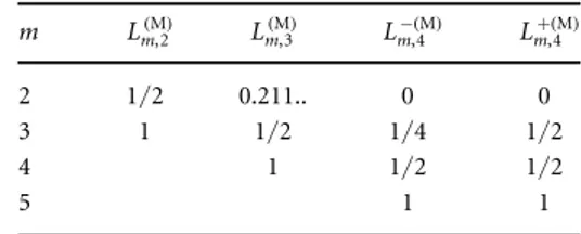
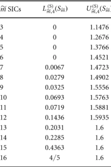
Table B5. Form~SIC states in_4_,

suboptimal lower and upper bounds, denoted by L_m,4Sm S ~( )₍ ~_{)andU S} m,4 m S ~( )₍ ~_{), are}

presented, for the quantityI_m,4S ~( ). These bounds are satisfied for all separable states, provided a specific subsetSm~of

m~SIC vectors is chosen from the SIC-POVM generated by thefiducial vector of equation(B.43). The subsets we

apply are given below equation(B.43). m~SICs L_m~( )S,4(Sm~) Um~( )S,4(Sm~) 3 0 1.1476 4 0 1.2676 5 0 1.3766 6 0 1.4521 7 0.0067 1.4723 8 0.0279 1.4902 9 0.0325 1.5556 10 0.0693 1.5763 11 0.0719 1.5881 12 0.1436 1.5935 13 0.2031 1.6 14 0.2285 1.6 15 0.4363 1.6 16 4_/5 1.6

L_{m d}~-_,( )S I_{m d}~( )S_, (ssep)U_{m d}+~_,( )S, (C.2) where the values L_{m d}~-_,( )S andU_{m d}~+_,( )S are given in tablesB3andB4, for dimensions d=2, 3, respectively. Note that

in d=2, L_{m d}~-_,( )S =L_{m d}~( )S_, and U_{m d}~+_,( )S =U_{m d}~( )S_, . For d=3 we can derive tighter upper and lower bounds

L_m,3S I_mS_,3 sep U_m,3, C.3

S

 s 

+

-~( ) ~( )( ) ~( ) ( )

as summarized in tableB4. However, equation(C.3) only applies for a specific set ofm~SIC vectors, which we have specified explicitly in the derivations above. For d=4 we are unable to find upper and lower bounds which apply for any subset ofm~SIC vectors, however, we dofind suboptimal bounds which apply for a specified set of

m~SIC vectors, namely

L_{m d}0 S_, I_{m d}S_, sep U_{m d}, , C.4

0 S

 s 

~( ) ~( )( ) ~( ) ( )

where the bounds are given in tableB5. To apply these bounds experimentally, it is required that the measurements correspond to the specified set of SIC vectors.

We will also prove later that for a complete set of d( +1)MUBs and d2SIC vectors, which correspond to quantum 2-designs, the bounds simplify to

I 1  _d( )M+_1,d(ssep)  2, (C.5) and d d I d d 1 2 1. C.6 d d, S sep 2  s  + ( ) + ( ) ( )

We now show that the inequalities above, for I_{m d}( )M_{, and}

I_{m d}~( )S_, , detect a larger set of entangled states as the number of measurements m increases. In particular, we highlight the following result:

Remark 1. As more MUBs and SIC vectors are applied to the detection criterion, the stronger the capability of detecting entangled states.

For a graphical illustration of this phenomenon we refer the reader tofigures2andC1. C.1. Examples: symmetric states

To demonstrate the observation made in remark 1, we consider a particular class of bipartite

d´d

( )-dimensional quantum states, the so-called symmetric states, and analyse their behaviour with respect to our detection criterion. Thefirst set of states we investigate are the Werner states

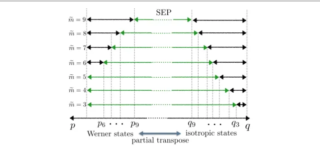
Figure C1. Inequalities for I2,3( )S, I3,3( )S, and I4,3( )S are applied to detect the entangled Werner and isotropic states defined in equations (C.7)

and(C.8). The upper₍U_{m d~}-_,( )S_{)and lower L}

m d, S + ~

( ( ))_{bounds can be found in tableB4. Green coloured lines show the range of states}

satisfying the inequalities, including all separable states. Lower bounds are violated by entangled Werner states and upper bounds by entangled isotropic states, with the critical values for the parameter p and q given as: p₆=0.11, p₇=0.13, p₈=0.28, p₉=0.5,