Re-visiting Riemannian geometry of symmetric positive definite matrices for the analysis of functional connectivity

ContentslistsavailableatScienceDirect

NeuroImage

journalhomepage:www.elsevier.com/locate/neuroimage

Re-visiting

Riemannian

geometry

of

symmetric

positive

definite

matrices

for

the

analysis

of

functional

connectivity

Kisung

You

_,

_Hae-Jeong

_Park

a Department of Applied and Computational Mathematics and Statistics, University of Notre Dame, Notre Dame, IN, USA b Department of Nuclear Medicine, Yonsei University College of Medicine, Seoul, Republic of Korea

c BK21 PLUS Project for Medical Science, Yonsei University College of Medicine, Seoul, Republic of Korea d Department of Cognitive Science, Yonsei University, Seoul, Republic of Korea

e Center for Systems Brain Sciences, Institute of Human Complexity and Systems Science, Yonsei University, Seoul, 50-1, Yonsei-ro, Sinchon-dong, Seodaemun-gu, Seoul 03722 Republic of Korea

a

r

t

i

c

l

e

i

n

f

o

Functional connectivity Riemannian manifold Symmetric positive definite Principal geodesic analysis

a

b

s

t

r

a

c

t

Common representations of functional networks of resting state fMRI time series, including covariance, precision, and cross-correlation matrices, belong to the family of symmetric positive definite (SPD) matrices forming a special mathematical structure called Riemannian manifold. Due to its geometric properties, the analysis and operation of functional connectivity matrices may well be performed on the Riemannian manifold of the SPD space. Analysis of functional networks on the SPD space takes account of all the pairwise interactions (edges) as a whole, which differs from the conventional rationale of considering edges as independent from each other. Despite its geometric characteristics, only a few studies have been conducted for functional network analysis on the SPD manifold and inference methods specialized for connectivity analysis on the SPD manifold are rarely found. The current study aims to show the significance of connectivity analysis on the SPD space and introduce inference algorithms on the SPD manifold, such as regression analysis of functional networks in association with behaviors, principal geodesic analysis, clustering, state transition analysis of dynamic functional networks and statistical tests for network equality on the SPD manifold. We applied the proposed methods to both simulated data and experimental resting state fMRI data from the human connectome project and argue the importance of analyzing functional networks under the SPD geometry. All the algorithms for numerical operations and inferences on the SPD manifold are implemented as a MATLAB library, called SPDtoolbox, for public use to expediate functional network analysis on the right geometry.

1. Introduction

Theprevailing view on thebrain is a highly-organized network, composedofinteractionsamongdistributedbrainregions.Interactions amongdistributedbrainregionsareoftencharacterizedbythe cross-correlationmatrixofspontaneousfluctuationsobservedintheresting statefunctionalmagneticresonanceimaging(rs-fMRI)(Biswaletal., 1995).The correlation matrix- a representation of functionalbrain network- hasserved asa basis fordiverse fields of brainresearch. Theexemplaryareasincludeexplorationofbraindiseasesusing func-tionalconnectivity(Drysdaleetal.,2017;Jangetal.,2016;Leeetal., 2017; Yahata et al., 2016), behaviorally associated brain networks (Kyeong etal.,2014; Smithetal.,2015),dynamicconnectivity anal-ysis(Allenetal.,2014;Calhounetal.,2014;ChangandGlover,2010;

∗_{Corresponding author at: Department of Nuclear Medicine, Yonsei University College of Medicine, Yonsei-ro 50-1, Sinchon-dong, Seodaemun-gu, Seoul, 03722,}

Republic of Korea.

E-mailaddress:parkhj@yonsei.ac.kr(H.-J. Park).

1 _{These authors equally contributed.}

Cribbenetal.,2012;Handwerkeretal.,2012;Hutchisonetal.,2013; Jeongetal.,2016;Montietal.,2014;Pretietal.,2017),identificationof individuals(Finnetal.,2015),inter-individualvariability(Jangetal., 2017) andbiomarkers in machinelearning (Dosenbach etal., 2010; Drysdale et al., 2017; Finn et al., 2015; Yahata et al., 2016). Par-tialcorrelationanalysis(inversecovariancematrix)hasalsobeenused (Choetal.,2017;Leeetal.,2017;Qiuetal.,2015)toexclude pseudo-connectivity(spurious connectionduetopolysynapticormodulatory effects).Inthosestudies,researchershaveanalyzedthecorrelation ma-tricesedgebyedge(elementofcorrelationmatrix)byconsideringeach edgeindependentlyfromotheredges(Dosenbachetal.,2010; Siman-Tovetal.,2016)orbyconsideringmultipleedgestogethertoexplain certaindependentvariables(Leonardietal.,2013;Parketal.,2014), particularly,inamachinelearningframework(Drysdaleetal.,2017; Yahataetal.,2016).Allthesedirectionsdonotmuch differin

disre-https://doi.org/10.1016/j.neuroimage.2020.117464

Received 23 January 2020; Received in revised form 4 August 2020; Accepted 12 October 2020 Available online 17 October 2020

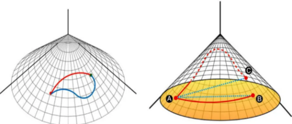
Fig. 1. General SPD manifold. The geodesic distance between A and B is shorter than that of A and C while it is reverse in the Euclidean distance.

gardingthetopologicaldependencyacrosselements,atypicalproperty ofthecorrelationmatrix.

Mathematically speaking,well-knownforms of representation for functionalconnectivity,such ascovarianceandprecisionalong with correlation,aresymmetricandpositivedefinite(SPD)matricesin com-mon.ItiswellknownthatthecollectionofSPDmatricesformsa cone-shapeRiemannianmanifold(Fig.1).Accordingly,theoperationsonthe SPDmanifoldcanbetterbeperformedbasedonthecorresponding ge-ometricstructureratherthantheEuclideangeometry.Thegeometric propertiesofSPDmanifoldhavenotyetbeenfullyrecognizedin neu-roimagingcommunities.Relativelyfewbutincreasingnumberof stud-iesonthefunctionalconnectivityhavebeenconductedonthespace ofSPDmatrices,includingevaluatingaverageandvariabilityofgroup levelcovariancematrices(Varoquauxetal.,2010;Yaminetal.,2019), statisticaltesting(Ginestetetal.,2017;Varoquauxetal.,2010),change pointdetection(Daietal.,2016),estimationofindividualcovariance matrix(Rahimetal.,2019),regressionoffunctionalconnectivityin es-timatingstructuralconnectivity(Deligiannietal.,2011)anddimension reductionsformachinelearning(Davoudietal.,2017;Ngetal.,2014; Qiuetal.,2015;Xieetal.,2017)tonameafew.

DespiteincreasinginterestforSPD-basedanalysis,westilllackaccess todiversemethodsforconnectivityanalysisontheSPDmanifold,such assmoothingandregression,clustering,principalcomponentanalysis, statetransitionanalysisofdynamicfunctionalnetworksandstatistical tests.Thepurposeofthecurrentstudyistoprovidemethodsfor ana-lyzingcorrelations(orcovariance,inversecovariancematrices)onthe SPDmanifold.Wewouldliketomentiononenotablecharacteristicof correlationmatrices.Correlationmatrix,whichisalsosymmetricand positivedefinite,isanormalizedversionofcovariancematrixand con-stitutesastrictsubsetorsubmanifoldofSPD.Tostudydistinctstructure intheconstrained set,geometryof elliptoperather thanSPD canbe asuitablecandidatetostudycorrelationmatrices.However,itmainly dealswithlow-rankstructureandhaslittlebeeninvestigated(Grubišić andPietersz,2007).Inthisstudy,weconsiderthecorrelationasa con-strainedtypeofSPDmatrixthatformsasubmanifold,inheriting geo-metricpropertiesofgeneralSPDmanifold.Thisdoesnotdiminishthe importanceof SPDmanifoldandourcontributiontostudyfunctional connectivitysincemanyrepresentationsoffunctionalconnectivityare equippedwithSPDpropertiesandtheproposedmethodsarepresented forabroaderclassofSPDmatrices.

Thecurrentpaperiscomposedoffourmainparts.Firstly,weprovide abriefoverviewanddescriptiononthemanifoldofSPDmatriceswith afocusonthecorrelationmatrix.Second,weintroducefunctionsfor operationsorlearningalgorithmsforcorrelationmatricesontheSPD manifoldinconsiderationofpracticalusagesinthefunctionalnetwork analysis.Thebasicoperationstartswithdefinitionofgeodesicdistance betweenSPDmatrices,whichbasesevaluationofgroupmean,variation, andstatisticaltestsontheSPDmanifold.Wealsointroducemethodsfor smoothingandregression,principal geodesicanalysisandclustering. Third,wepresenttheneedtofunctionalconnectivitymatricesonthe SPDspacebysimulationandbyexperimentaldata.Allthealgorithms areimplementedintermsofMATLAB(Mathworks,inc.USA)toolbox,

calledSPDtoolbox,whichisfreelyavailableonGitHub(https://github. com/kyoustat/papers) forpublicuse toexpediatefunctionalnetwork analysisontherightgeometry.

2. Methods

2.1. ReviewofRiemanniangeometry 2.1.1. ElementsofRiemannianmanifold

Inbrief,amanifoldisatopologicalspacethatlocallyresembles Euclideanspaceateachpoint.Manifoldiscalledsmoothwhen transi-tionmapsaresmooth.ARiemannianmanifold(𝑀,𝑔)isasmooth man-ifoldwhoseinnerproduct𝑔𝑝onthetangentspaceforapointpvaries smoothly.Fromapractitioner’sperspective,itisimportanttokeepin mindthatRiemannianmanifoldisnotavectorspace.Thatmeans,we areendowedwithaconceptofdistancethatsatisfiesmetricproperties onthespacethatislocallyEuclidean-alikebutitisnotEuclideanspace. Forexample,consideroperationsonasphere𝑆2_{⊂ ℝ}3_andtakenorth

andsouthpoles withcoordinates(0,0,1)and(0,0,-1). Ifwe sim-plytreatdataresidingonthesurfacewithEuclideanstructure, averag-ingcoordinatesofnorthandsouthpoleswouldreturn(0,0,0),which correspondstotheinnercoreororiginofthesphere.However,ifwe wantmathematicaloperationstoabidebythesphericalgeometry, sim-ply’adding’coordinatesoftwopoleswouldbeaninvalidconcept.We introducesomeconceptsanddefinitionswithoutrigorousmathematical expositioninthefollowing.

Atangentspace𝑇𝑝atapoint𝑝∈isasetoftangentvectors (Fig.2),whicharederivativesofcurvescrossingp.Thestatementfora manifoldbeinglocallysimilartoEuclideanspacegenerallyreferstothe tangentspaceanditspropertiesasvectorspace.Twoimportant math-ematicaloperationsareexponentialandlogarithmmaps.Let𝑣∈𝑇_𝑥 beatangentvectoratx.Exponentialmap𝑒𝑥𝑝𝑥(𝑦)∈definesaunique shortestcurve(geodesic)fromapointxinthedirectionofvinso thattheoperationresultsinapointin(Fig.2).Logarithmmapisan inverseofexponentialmapinthatfor𝑥,𝑦∈,𝑙𝑜𝑔𝑥(𝑦)∈𝑇𝑥which correspondstoywhensentbackviaexponentialmap.Finally,geodesic distanceisthelengthoftheshortestcurvethatconnectstwopointsx

andy.

2.1.2. Fréchetmeanandvariation

Giventhedata𝑥1,𝑥2,…,𝑥𝑛∈,thesampleFréchetmean𝜇𝑛is de-finedasaminimizerofthesumofsquareddistances,

𝜇𝑛=argmin 𝑝∈ 1 𝑛 𝑛 ∑ 𝑖=1 𝜌2(_𝑝,𝑥 𝑖)

where𝜌 ∶×→ (ℝ)isageodesicdistanceforx,y∈M,thelength oftheshortestcurveonMconnectingtwopoints.IfFréchetmeanexists, theFréchetvariation𝑉𝑛istheattainedminimumvaluefor𝜇𝑛,

𝑉𝑛= 1_𝑛 𝑛 ∑ 𝑖=1 𝜌2(_𝜇 𝑛,𝑥𝑖)

2.1.3. Riemannianmetricandgeodesicdistance

Riemannianmetricgisasymmetric(0,2)-tensorfieldthatis positive-definiteateverypoint.Formallyspeaking,wehave

𝑔𝑝∶𝑇𝑝×𝑇𝑝→ (ℝ),𝑝∈

suchthatforeverydifferentialvectorfieldsX,YonM,𝑝↦ 𝑔𝑝(𝑋|𝑝,𝑌|𝑝)is asmoothfunctionand𝑔(𝑋,𝑋)|_𝑝∶=𝑔_𝑝(𝑋|_𝑝,𝑋|_𝑝)>=0and𝑔(𝑋,𝑋)|_𝑝=0 ifandonlyif𝑋|𝑝=0.Locallyatapointp,itendowsaninnerproduct structureontangentspace.Oneobservation(Pennec,2006)isthatthe geodesicdistanceiscloselyrelatedtotheRiemannianmetricinthatfor

x,y∈M, 𝜌(𝑥,𝑦)= min 𝛾∶[0,1]→∫ 1 0 ̇𝛾(𝑡 )dt=‖lo𝑔_𝑥(𝑦)‖ = √ 𝑔𝑥(lo𝑔𝑥(𝑦),lo𝑔𝑥(𝑦)) for𝛾 isacurveminimizingthedistanceandlogarithmicmaplo𝑔_𝑝(⋅)∶ → 𝑇𝑝.

2.2. SPDmanifold

OurspecialinterestisthespaceofSPDtowhichmost representa-tionsoffunctionalconnectivitybelong.Conventionalmeasuressuchas

covariance,precision,andcorrelationmatricesallshareidentical proper-ties.

Definition. SPD(n)is aspaceofsymmetricandpositivedefinite ma-tricesSPD(𝑛)={𝑋∈ℝ𝑛×𝑛_|𝑋=𝑋⊤_,𝜆

min(𝑋)>0}where𝜆𝑚𝑖𝑛denotesthe minimumeigenvalue.

ItiswellknownthatSPDis,infact,aRiemannianmanifold.That means,thereexistscertaingeometricstructuresnotnecessarilysimilar tothatofEuclideanspace.Inthefollowingsections,weprovide math-ematicalcharacterizationandcomputationalissuesfrompedagogical perspective.

2.2.1. Matrixexponentialandlogarithm

ForasquarematrixX,thematrixexponentialisdefinedas

Exp(𝑋)∶= ∞ ∑ 𝑘=0 1 𝑘!𝑋 𝑘

analogoustoareal-numbercase.Matrix(principal)logarithmcanalso bedefinedusingthedefinitionaboveby

𝐿𝑜𝑔(𝑋)∶=𝑌 suchthat𝐸𝑥𝑝(𝑌)=𝑋.

Formoredetailsofmatrixexponential,logarithm,andtheirrolesin whatisknownasLiegroupinconnectionwithSPDmanifold,werefer toMoakher(2005) forinterestedreaders.

Due to its pervasive nature, the space of SPD matrices has been extensively studied (Bhatia, 2015). Many attempts to formal-izethe non-Euclideangeometryon SPD havebeen madewhere dis-tance between two SPD objects are defined by Cholesky decom-position (Dryden et al., 2009), symmetrized Kullback-Leibler diver-gence(WangandVemuri,2005),Jensen-BregmanLogDetdivergence (Cherianetal.,2013)andWassersteindistance(Takatsu,2011)toname afew.Amongmanyframeworks,themostpopularmetricsontheSPD geometricspacearetheaffine-invariantRiemannianmetric(AIRM)and thelog-EuclideanRiemannianmetric(LERM).

2.2.2. IntrinsicgeometrywithAIRM

Affine-invariantRiemannianmetric(AIRM)isoneofthemost pop-ulargeometricstructuresonthespaceofSPDmatrices(Pennecetal., 2006).Asitsnamesuggests,thespecificmetric,whichtakestwo ele-mentsinatangentspacetoreturnanumber,characterizesthe corre-spondinggeometryofthespace.ForSPDequippedwithAIRM,given twotangentvectors𝑣,𝑤atapoint𝑝∈=SPD,

𝑔𝑝(𝑣,𝑤)=<𝑣,𝑤>𝑝∶=Tr(𝑝−1𝑣𝑝−1𝑤)

where𝑝−1_{isstandardmatrixinverseandTratraceoperator.}

Twoimportantoperationsthatconnectthemanifoldandthe tan-gentplane𝑇𝑥atapoint𝑥∈ areexponentialandlogarithmicmaps forwhichSPDmanifoldisendowedanalyticalformula.Foratangent vector𝑣at𝑥,itsexponentialmap𝑒𝑥𝑝𝑥∶𝑇𝑥→ isdefinedas

𝑒𝑥𝑝𝑥(𝑣)=𝑥1∕2_𝐸𝑥𝑝(_𝑥−1∕2_𝑣𝑥−1∕2)_𝑥1∕2

andlogarithmicmapat𝑥,𝑙𝑜𝑔𝑥∶→ 𝑇𝑥forapoint𝑦∈is

𝑙𝑜𝑔𝑥(𝑦)=𝑥1∕2𝐿𝑜𝑔(𝑥−1∕2𝑦𝑥−1∕2)𝑥1∕2

sothatthegeodesicdistance𝑑∶ × → ℝ+fortwopoints𝑥,𝑦∈

=𝑆𝑃𝐷 canbecomputedas

𝑑2_{(𝑥,𝑦)=𝑔}

𝑥(𝑙𝑜𝑔𝑥(𝑦),𝑙𝑜𝑔_𝑥(𝑦))=∥𝐿𝑜𝑔(𝑥−1𝑦)∥2_𝐹.

2.2.3. ExtrinsicgeometryunderLERM

The log-EuclideanRiemannianmetric (LERM)is anotherpopular machineryalongwithAIRM(Arsignyetal.,2007).Tobrieflyintroduce, LERMframeworkcanbeconsideredasananalysisprocedureby embed-dingpointsinSPDmanifoldtoEuclideanspaceviamatrixlogarithm.For example,geodesicdistancefortwopoints𝑥,𝑦∈=𝑆𝑃𝐷 underLERM isdefinedas

𝑑2_{(𝑥,𝑦)=∥𝐿𝑜𝑔(𝑥)−𝐿𝑜𝑔(𝑦)∥}2

𝐹,

with∥⋅∥_𝐹 aFrobeniusnorm.Aswenotedbefore,LERMaccountsfor EuclideangeometryafterthematrixlogarithmattheidentityI.Wecan checkthisstatementbythefactthat𝐿𝑜𝑔(𝑥)=𝑙𝑜𝑔_𝐼(𝑥)withconventional innerproductintheEuclideanspace.

Weclosethis sectionbymaking anotethatAIRMandLERMare twoprincipledapproachesknownasintrinsicandextrinsicanalysisof manifold-valueddata.Whileintrinsicapproachisstrictlyboundbythe innate geometric conditionsand makes all procedures more persua-sive,extrinsicapproachdependsonanembeddingtoEuclideanspace that preserves considerableamount ofgeometricinformation, which easescomputationandtheoreticalanalysisthereafter.Thedichotomy is commonin the studiesof statistics on manifolds and we suggest (Bhattacharya andBhattacharya, 2012) tointerested readersfor de-taileddescriptionofthedichotomyofprincipledapproaches.

2.3. AlgorithmsontheSPDmanifold

Inthissection,severallearningandinferencefunctionsaredescribed withalgorithmicdetails.Acrossalldescriptionsinthissection,weuse thefollowingnotations;{𝑋_𝑖}𝑛_𝑖=1∈fordataresidingontheSPD man-ifold,𝜇 and𝜇𝑗 meansof alldataandclassj,Si anindexsetof data who belongto the cluster classi, superscript (t) _{an iteration t, and} 𝑑∶ × → ℝ+ageodesicdistancefunctionasdefinedinthe

pre-vious section.Algorithmsintroduced in this sectionare largely gov-ernedbytheintrinsicgeometryofAIRMframework.Forextrinsic log-Euclideangeometry,mostofstandardalgorithmsfordatainEuclidean spacecanbedirectlyapplicableaftertakingmatrixlogarithmic trans-formationonalldatapointsaslongasthefinaloutputmatrixinthe Euclideanspaceistakenbackviamatrixexponential.

2.3.1. Fréchetmeanandvariation(spd_mean.m)

Given data points 𝑥𝑖∈,𝑖=1,…,𝑛, empirical intrinsic Fréchet mean𝜇𝑛isaminimizerofaveragesquaredgeodesicdistances

𝜇𝑛=argmin 𝑝∈ 1 𝑛 𝑛 ∑ 𝑖=1 𝑑2(_𝑝,𝑥 𝑖)=∶𝑓(𝑝)

andcorrespondingvariationis 𝑉𝑛= 𝑛 ∑ 𝑖=1 𝑑2(_𝜇 𝑛,𝑥𝑖)∕𝑛.

Oneofstandardmethodstoobtain𝜇𝑛istouseaRiemanniangradient descentalgorithmproposedinPennecetal.(2006),inwhichconditions forexistence anduniquenessarediscussedaswellas thealgorithm. Ateachiteration,thegradientof𝑓 iscomputedinanambientspace ∇𝑓(𝑝)=∑𝑛_𝑖=12𝑙𝑜𝑔_𝑝(𝑥_𝑖)∕𝑛andthenprojectedbackontothemanifoldby exponentialmapsothatwerepeatfollowingstepsatiteration𝑡,

𝑊(𝑡)₌ 2 𝑛 𝑛 ∑ 𝑖=1 𝑙𝑜𝑔𝜇(𝑡)(𝑥_𝑖) 𝜇(𝑡+1)_{=𝑒𝑥𝑝} 𝜇(𝑡)(−𝑊(𝑡))

untilconvergenceandtheobtainedmean𝜇𝑛ispluggedintoobtainthe correspondingvariationofourdata.

Ontheotherhand,computationofextrinsicFréchetmeanand vari-ationunderlog-Euclideangeometryisratherstraightforward.As men-tionedbefore,underLERMframework,dataareembeddedintosome Euclideanspacebymatrixlogarithmicmapinthatwehavethe follow-ingone-linerexpressiontocomputeobjectsofourinterests,

𝜇𝑛=Exp ( 1 𝑛 𝑛 ∑ 𝑖=1 Log(𝑥_𝑖) ) 𝑉𝑛= 1_𝑛 𝑛 ∑ 𝑖=1 ‖Log(𝜇𝑛)−Log(𝑥𝑖)‖2 ,

where∥⋅∥ isaconventionalEuclideannorm.

2.3.2. Testforequalityoftwodistributions(spd_eqtest.m)

Itisoftenaprerequisitetocheckwhethertwogroupsofobjectsare identicallydistributedforfurtheranalysis.Instatistics,thisisusually conveyedwithhypothesistestingprocedurestodetermineifthere ex-istsdifferenceincertainmeasuresofinterests,includingmean,variance, andsoon.Oneofgeneraltestmethodsisatwo-sampletestingforthe equalityoftwodistributions.Whengiventwosetsofindependent ob-servations𝑥1,…,𝑥𝑚∼𝐹 and𝑦1,…,𝑦𝑛∼𝐺,wetestthenullhypothesis

𝐻0∶𝐹 =𝐺 againstthealternative𝐻1∶𝐹 ≠ 𝐺.

Among many classes of distribution tests developed for Eu-clidean data, we employ one nonparametric method by Biswasand Ghosh(2014).Thismethodissolelybasedoninter-pointdistances be-tweendatapointsforinference.Maaetal.(1996) showedthattesting

𝐹=𝐺 isequivalenttotestwhetherthreedistributions𝐷𝐹 𝐹,𝐷𝐹 𝐺,𝐷𝐺𝐺 areidentical,where𝐷𝐹 𝐹,𝐷𝐹 𝐺,𝐷𝐺𝐺 denotethedistributionsof∥𝑋−

𝑋∗∥,∥𝑋−𝑌∥,and∥𝑌−𝑌∗∥with𝑋∗and𝑌∗beingidenticallydistributed

as𝑋 and𝑌.TheprooffromMaaetal.(1996) isdirectlyapplicableto RiemannianmanifoldsembeddedinEuclideanspacesincethelimitin volumeformcoincideswithEuclideanballlocally.Thisleadstoa conve-nientadaptationofthemethodbysimplyreplacingtheEuclideannorm withgeodesicdistanceonSPD.Tobrieflyintroducetheadaptationof aforementionedmethod,define

̂𝜇𝐷𝐹 = [ 2 𝑚(𝑚−1) 𝑚 ∑ 𝑖=1 𝑚 ∑ 𝑗=𝑖+1 𝑑(𝑥𝑖,𝑥𝑗), _𝑚𝑛1 𝑚 ∑ 𝑖=1 𝑛 ∑ 𝑗=1 𝑑(𝑥𝑖,𝑦𝑗) ] ̂𝜇𝐷𝐺 = [ 1 𝑚𝑛 𝑚 ∑ 𝑖=1 𝑛 ∑ 𝑗=1𝑑 ( 𝑥𝑖,𝑦𝑗), _𝑛(𝑛2₋₁₎ 𝑛 ∑ 𝑖=1 𝑛 ∑ 𝑗=𝑖+1 𝑑(𝑦𝑖,𝑦𝑗) ]

andrejectthenullhypothesis𝐻0∶𝐹=𝐺 forlargervaluesofthetest

statistic𝑇𝑚,𝑛=‖ ̂𝜇_𝐷𝐹− ̂𝜇_𝐷𝐺‖2₂.Sinceanalyticalexpressionforthe sam-plingdistributionof𝑇_𝑚,𝑛inthelimitingsenseisnotavailable,weuse the permutation test by rearranging labels of the givendata in or-dertoachieveasuitablethresholddefining‘largeness’ofthestatistic (Pitman,1937).Incomputationalaspect,oncewehaveapre-computed distancematrix𝐷𝐹 𝐺∈ℝ{𝑚+𝑛}× {𝑚+𝑛}forallobservations,permutation testingproceduredescribedabovedoesnotdemandintensive comput-ingresourcessinceacquiring𝑇_𝑚,𝑛consistsofscalaradditionand multi-plicationonly.

2.3.3. Pairwisecoefficienttestofequaldistribution(spd_eqtestelem.m)

Infunctionalconnectivityanalysis, itisoftenof interesttolocate whichconnectionsshowgroup-leveldifferenceatitssignificance.One commonapproachistoperformunivariatetwo-sampletestingforeach entryandapplymultipletestingcorrection.Kimetal.(2014)compared performanceofsomestatisticalhypothesistestsindetectinggroup dif-ferencesinbrainfunctionalnetworks.Theaforementionedapproachto employmultipleunivariatetestsisbasedonanimplicitassumptionthat eachtestforpairwisecoefficientsisindependentofeachother. Further-more,asymptotic-basedtestsdependuponadditionalassumptions in-cludingunderlyingdistributioninthatabsenceofsufficientvalidation necessitatestheuseofnonparametricprocedure(Wasserman,2006).

Inthisstudy,weintroduceanovelprocedureforcomparing pair-wisecoefficientsundergeometricconstraintsimposedbySPDmanifold. Hutchisonetal.(2010) proposedabootstrapprocedureforcomparing coefficientsatthevicinityofFréchetmeansbylogarithmicmappingto assureindependenceofparameters.Insteadoflocalcomparison,wetake analternativeapproachtousegroup-levelinformationrepresentedby Fréchetmeanandcompareelementsthereafterusingpermutation test-ingframework.Givendataoftwogroups𝑥1,…,𝑥𝑚and𝑦1,…,𝑦𝑛allon SPD(𝑝),thealgorithmgoesasfollows.

1 computeFréchetmeans𝜇_𝑥and𝜇_𝑦andtake𝐷xy=|𝜇𝑥−𝜇𝑦| ∈ (ℝ)𝑝×𝑝. 2 For𝑡=1,…,𝑇iterations,

(a) select̃𝑥1,…,̃𝑥𝑚and̃𝑦1,…,̃𝑦𝑛fromthedatawithoutreplacement. (b) computeFréchetmeans𝜇_̃𝑥,𝜇_̃𝑦forpermutedsamples

(c) record𝐷(𝑡)

𝑥𝑦=|𝜇_̃𝑥−𝜇_̃𝑦|

3 foreach(𝑖,𝑗)pair,compute𝑝-values𝑝(𝑖,𝑗)by

𝑝(𝑖,𝑗)= #{𝑧∈𝐷1∶𝑇 xy (𝑖,𝑗)|𝑧≥𝐷xy(𝑖,𝑗) } +1 𝑇+1 where𝐷1∶𝑇 𝑥𝑦 (𝑖,𝑗)=[𝐷1𝑥𝑦(𝑖,𝑗),…,𝐷𝑇𝑥𝑦(𝑖,𝑗)].

2.3.4. k-meansclustering(spd_kmeans.m)

k-meansalgorithm(MacQueen,1967)is oneoffamousclustering algorithmsfordataanalysis.AspointedoutinGohandVidal(2008), themethodiseasilyextensibletonon-Euclideandatasinceitsolely de-pendsonthedistancemeasureindeterminingclassmemberships.We implementedstandardLlyod’salgorithm(Lloyd,1982)modifiedtoour context.

1 randomlychoosekdatapointsasclustermeans𝜇(1) 1 ,…,𝜇

(1)

𝑘 . 2 repeatfollowingstepsuntilconvergence:

• assigneachobservationtotheclusterbysmallestdistancesto clustercenters, 𝑆(𝑡) 𝑖 ={𝑋𝑖|𝑑 ( 𝑋𝑖,𝜇𝑖(𝑡) ) ≤𝑑(𝑋𝑖,𝜇(𝑗𝑡) ) forall𝑗,1≤𝑗≤𝑘}

andwhenitcomestoasituationwhereanobservationcanbelong tooneofmultipleclusters,assigntheclusterrandomly. • updateclustercentroidsbyFréchetmeansofeachclass,

𝜇(𝑡+1) 𝑖 =argmin_𝑝∈𝑀 ∑ 𝑗∈𝑆(𝑡) 𝑖 𝑑2(_𝑝,𝑋 𝑗)for𝑖=1,…,𝑘 where|𝑆𝑖| referstothenumberofobservationsinclassi.

Toguidetheselectionofclusternumbersk,weimplementan adap-tation ofcelebrated Silhouettemethod (Rousseeuw, 1987)asa clus-ter quality score metric since it only relies on any distance metric (spd_clustval.m ).Silhouetteisameasureofproximityforobservations inaclustertothepointsinitsneighboringclusters.Eachobservation ismeasuredwithascorebetween[−1,1]wherelargepositivenumber indicatesanobservationiswellseparatedbythecurrentclustering.For eachobservationi,asilhouettevalueis

𝑠(𝑖)= 𝑏(𝑖)−𝑎(𝑖) 𝑚𝑎𝑥{𝑎(𝑖),𝑏(𝑖)} where 𝑎(𝑖)= 1 ||𝑆𝑖|| −1 ∑ 𝑗∈𝑆𝑖,𝑖≠𝑗 𝑑(𝑋𝑖,𝑋𝑗)

𝑏(𝑖)=min 𝑖≠𝑗 1 || |𝑆𝑗||_| ∑ 𝑗∈𝑆𝑗 𝑑(𝑋𝑖,𝑋𝑗)

Fromtheexpressionabove,a(i)istheaveragedistancebetweenan ob-servationiandtherestinthesameclusterofXi,whileb(i)measuresthe

smallestaveragedistancefromi-thobservationtoallpointsinallother clusters.Whenaclusterissingletonconsistingofasingleobservation, sets(i)=0.Oncesilhouettevaluesarecomputedforalldatapoints, globalscoreiscomputedbyaveragingindividualsilhouettevaluesand apartitionofthelargestaveragescoreissaidtobesuperiortoothers.

2.3.5. Modularity-basedclustering

Itshouldbenotedthateveryexecutionofk-meansclusteringshows variationsin itsresultdue toinitialization.Tomake aconsistent re-sultformultiplek-meansclusteringandthusmakeclusteringrobustto initialvalues,weadoptmodularityanalysisofmultiplek-means cluster-ing,whichwasappliedtosortneuraltimecoursesinourpreviousstudy (Jungetal.,2019).Thealgorithmrepeatsk-meansclusteringNtimesfor samplecovariancematriceswithanempiricalKorevaluatedby Silhou-ettescore.Then,itevaluatesthefrequencyforeachpairofcovariances beingasameclusteramongNtimesofk-meansclustering.This com-posesafrequencyadjacencymatrixforeverypairsofcovariance ma-trices.Theelementofthefrequencyadjacencymatrixdesignateshow frequentlytwonodes(covariances)areclusteredasasamecluster.The

modularityoptimizationalgorithm(NewmanandGirvan,2004), imple-mentedintheBrainConnectivityToolbox(RubinovandSporns,2010), identifiesoptimalclustersfromthefrequencyadjacencymatrixwhile maximizingthemodularityindexQ.ThemodularityindexQforan ad-jacencymatrixAisdefinedas:

𝑄= 1 𝑉 ∑ 𝑖𝑗 ( 𝐴𝑖𝑗−𝑠_𝑉𝑖𝑠𝑗 ) 𝛿𝑀𝑖𝑀𝑗

whereA_ijistheedgeweightbetweenthei-thandj-thnodes,Visthe totalsumofweights.𝛿𝑀𝑖𝑀𝑗 isakroneckerdeltafunctionthatassigns 1ifthei-thandj-thnodesareinthesamemodule(Mi =Mj)and0

otherwise.

Inadditiontok-meansclustering,theSPDtoolboxprovides cluster-ingofsamplecovariancematricesbyevaluatinganadjacencymatrixof negativegeometricdistancesamongthesamples.Themodularity opti-mizationalgorithmfindsclustersthatmaximizethemodularityindex.

2.3.6. Smoothingandregression(spd_smooth.m)

Supposewe havepaireddata(𝑡_𝑖,𝑋_𝑖),𝑖=1,…,𝑛where𝑡𝑖∈ℝ rep-resents one-dimensional covariate such as age or timeand 𝑋𝑖∈ manifold-valueddata.Oneofthemostfundamentalquestionswouldbe tomodeltherelationshipbetween𝑡and𝑋,i.e.,𝑋𝑖=𝐹(𝑡𝑖)+𝜖𝑖.This re-gressionframework,however,isnoteasilydefinedevenforparametric familyof𝐹(⋅)sincetheconceptofsubtractiononRiemannianmanifold maynotbestraightforward.Nevertheless,itisneedlesstoemphasize theimportanceofsuchproblemsincethelearnedregressionfunction maybeusedforprediction,smoothing,andsoon.

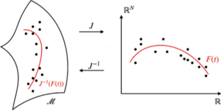
A fast yet powerful method was recently proposed by Lin et al. (2017) for manifold-valued response 𝑋∈ and vector-valuedexplanatoryvariable𝑡∈ℝ𝑝.Wefocusonintroducingaspecial case 𝑝=1 for simplicity along with its usage as a nonparametric regressionframeworkagainstone-dimensionalcovariate.Thekeyidea is to graft kernel regression (Nadaraya, 1964; Watson, 1964) onto log-Euclideangeometricstructure.

Let𝐽∶→ ℝ𝑁,𝑁≥dim()beanembeddingofourSPD mani-foldontohighdimensionalEuclideanspace(Fig.3).Aconvenient choice for 𝐽 is an equivariant embedding, which is known to pre-servesubstantialamountofgeometricstructure(Bhattacharyaand Bhat-tacharya,2012).ForSPDmanifold,theembeddingis𝐽(𝑋)=𝐿𝑜𝑔(𝑋), whichislogarithmicmappingof𝑋 atidentity𝐼,

𝐽(𝑋)=𝐿𝑜𝑔(𝑋)=𝐼1∕2_𝐿𝑜𝑔(_𝐼−1∕2_𝑋𝐼−1∕2)_𝐼1∕2_{=𝑙𝑜𝑔}

𝐼(𝑋)

Fig. 3. A schematic description of extrinsic local regression.

Fig. 4. A schematic description of principal geodesic analysis (PGA). whoseinverse𝐽−1_{isthereforeexponentialmapping.Giventwo}

map-pings,theextrinsickernelestimateoftheregressionfunction𝐹_𝐸 is de-finedas 𝐹𝐸(𝑡)=𝐽−1((𝐹(𝑡))) where 𝐹(𝑡)= 𝑛 ∑ 𝑖=1 𝐽(𝑋𝑖)𝐾ℎ(𝑡𝑖−𝑡) ∑𝑛 𝑗=1𝐾ℎ(𝑡𝑗−𝑡)

forakernelfunction𝐾ℎ(𝑧)=𝐾(𝑧∕ℎ)∕ℎwithapositivebandwidthℎ>0 thatcontrolsthedegreeofmassconcentrationandprojection∶ℝ𝑁→

𝐽(). Kernel bandwidth ℎ is either fixed or determined via cross-validation.SPDtoolboxprovidesk-foldcrossvalidationtodetermine op-timalℎ(spd_smoothcv.m ).

2.3.7. Principalgeodesicanalysis(spd_pga.m)

Principalcomponentanalysis(PCA)isawell-knownmethodfor ex-ploratorydataanalysis(Hotelling,1936;Pearson,1901).Toreviewin brevity, itaimsat findinga basisthat captures the largestvariance ontowhichthedataisprojected.Thisnatureallowsustoexploitthe methodfordimensionreductionandfeatureextraction.Givenadata matrix𝑋=[𝑥1| ⋯|𝑥𝑛]∈ℝ𝑝×𝑛whereeachrowhaszeromean,top

eigen-vectors𝑤𝑖,𝑖=1,…,𝑘,suchthatΣ𝑤𝑖=𝜆𝑖𝑤𝑖,𝜆1≥𝜆2≥…≥𝜆𝑝aretaken as basis where Σ =𝑋𝑋⊤∕𝑛 is an empiricalcovariance matrix. The reducedmatrix𝑌 =[𝑦1| ⋯|𝑦𝑛]∈ℝ𝑘×𝑛 isobtainedby𝑌 =𝑉⊤𝑋 where 𝑉 =[𝑣1| ⋯|𝑣𝑘]∈ℝ𝑝×𝑘isamatrixconsistingofeigenvectorsasabove -alsocalledasprincipalcomponentsorloadings.

Fletcheretal.(2004) graftedtheveryideaontothesettingwhere dataliesonmanifold.Sincethereisnodirectcounterpartofempirical covariancematrixandeigen-decompositiononRiemannianmanifold, alocalapproachwasfirsttaken.AfterobtainingaFréchetmean𝜇 for

givendata𝑋1,…,𝑋𝑛∈,everyobservationispulledbackontothe

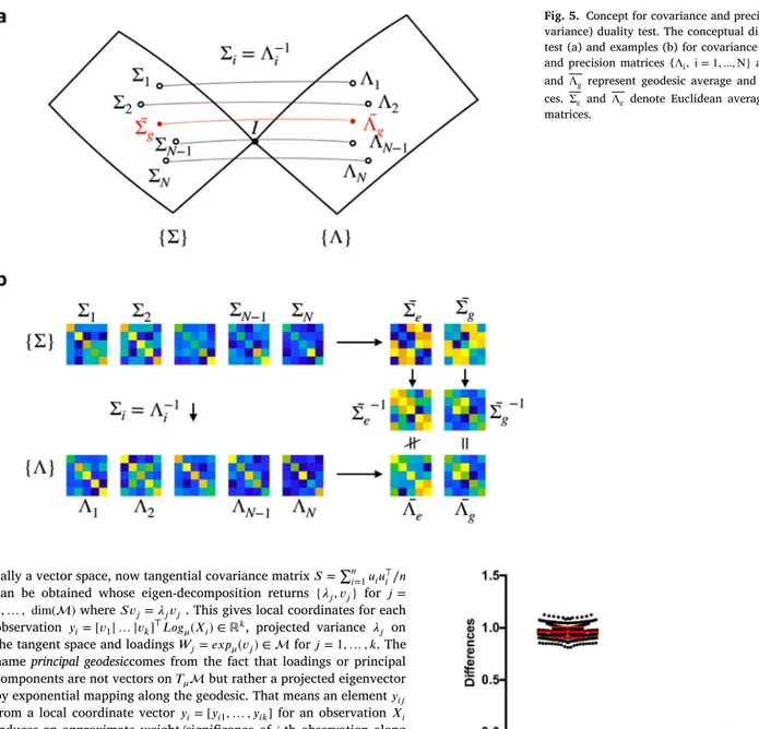
lo-Fig. 5. Concept for covariance and precision (inverse co- variance) duality test. The conceptual diagram of duality test (a) and examples (b) for covariance { Σi, i = 1 ,...,N}

and precision matrices { Λi, i = 1 ,...,N} are presented. Σg

and Λgrepresent geodesic average and precision matri-

ces. Σe and Λe denote Euclidean average and precision

matrices.

callyavectorspace,nowtangentialcovariancematrix𝑆=∑𝑛_𝑖=1𝑢_𝑖𝑢⊤_𝑖∕𝑛 can be obtained whose eigen-decompositionreturns {𝜆_𝑗,𝑣_𝑗} for 𝑗= 1,…, dim()where𝑆𝑣𝑗=𝜆_𝑗𝑣_𝑗 .Thisgiveslocalcoordinatesforeach observation 𝑦_𝑖=[𝑣1| … |𝑣𝑘]⊤𝐿𝑜𝑔𝜇(𝑋𝑖)∈ℝ𝑘, projected variance 𝜆𝑗 on thetangentspaceandloadings𝑊𝑗=𝑒𝑥𝑝𝜇(𝑣𝑗)∈for𝑗=1,…,𝑘.The nameprincipalgeodesiccomesfromthefactthatloadingsor principal componentsarenotvectorson𝑇_𝜇butratheraprojectedeigenvector byexponentialmappingalongthegeodesic.Thatmeansanelement𝑦𝑖𝑗 fromalocalcoordinatevector𝑦𝑖=[𝑦𝑖1,…,𝑦𝑖𝑘]foranobservation𝑋𝑖 inducesanapproximateweight/significanceof𝑖-thobservationalong

𝑗-thgeodesicdirection.Pleasenotethatprincipalgeodesics{𝑊_𝑖}𝑘_𝑖=1are notorthogonaltoeachotherasinconventionalPCAsothattheyshould beunderstoodasapproximatebasisinalocalsensearoundtheFréchet mean𝜇.

3. Results

3.1. Simulation1.WhySPDgeometryshouldbeused?

OtherthanmathematicalcharacterizationofSPDthatisclearly dif-ferentfromthatofavectorspace,wedescribewhythegeometryofSPD endowsanaturalinterpretationwithrespecttoanalysisof representa-tionsforfunctionalconnectivity.Assumewehaveapopulationof𝑁

co-varianceconnectivitymatrices{Σ}={Σ1,…,Σ𝑁}.Itisofofteninterest

toinvestigatepartialassociationamongdifferentROIsusingprecision matrices{Λ}={Λ1,…,Λ𝑁}whereeachΛ𝑖isaninversecovariance ma-trixΣ−1

𝑖 .ThatmeanswemusthaveΣ𝑖Λ𝑖=Λ𝑖Σ𝑖=𝐼 forall𝑖where𝐼 is anidentitymatrix.Thenitisnaturaltoquestionwhetheraverages ̄Σ and̄Λ alsosatisfytheaboverelationship̄Λ ̄Σ = ̄Σ ̄Λ =𝐼 aswell.Thisidea isrepresentedinFig.5 that ̄Λ isaninverseof_Σ.̄

IfweconsiderEuclideangeometry,thisisnotnecessarilytrue. Con-sidering{Σ} and{Λ} aselementsinEuclidean space,we candefine

Fig. 6. The result of covariance and precision (inverse covariance) reciprocity test. averagesasfollows ̄Σ = 1 𝑁 𝑁 ∑ 𝑖=1 Σ_𝑖and ̄Λ = 1 𝑁 𝑁 ∑ 𝑖=1 Λ_𝑖= 1 𝑁 𝑁 ∑ 𝑖=1 Σ−1_𝑖 inthat ̄Σ ̄Λ = 1 𝑁2 {_𝑁 ∑ 𝑖=1 Σ_𝑖Σ−1 𝑖 + ∑ 𝑖≠𝑗 Σ_𝑖Σ−1 𝑗 } = 1 𝑁2 { 𝑁𝐼+∑ 𝑖≠𝑗 Σ_𝑖Σ−1 𝑗 } .

Therefore,itisnotguaranteedthatEuclideanaveragesofcovariance andprecisionmatricesareinverseofeachotherunlessΣ_𝑖Σ−1

𝑗 =𝐼 forall

𝑖≠ 𝑗.

Ontheotherhand,averagesdefinedasFréchetmeansover{Σ} and {Λ}underthegeometryinducedbyAIRMsatisfytheabovestatement undermild conditions.Sincematrixinverseis abijectivemapwhile geodesicdistanceispreservedunderinversion,Fréchetmeanof preci-sionmatricesisaninverseofFréchetmeanofcovariancematricesifthe meanisunique.

Weempiricallyshowedhowthechoiceofgeometryand correspond-ingdefinitionof average/meanleadstotheconsistencywith our in-tuition.Wegenerated100covariancematricesΣ_𝑖,𝑖=1,…,100 identi-callyandindependentlyfromWishartdistribution𝑝(𝑉,𝑛)with𝑝=5 dimension(networksize),𝑛=20degreesoffreedom(thelengthoftime series)forstrictpositivedefiniteness,and𝑉 =𝐼5 ascalematrix.After

computingprecisionmatricesΛ_𝑖=Σ−1_𝑖 ,wecomputebothEuclideanand FréchetmeanswithbothAIRMandLERMframeworksoncovariance andprecisionmatricesrespectively.Foreachrun,thegapisobtainedas ∥ ̄Λ ̄Σ −𝐼5∥𝐹toseehowclose ̄Λ istōΣ−1where∥𝐴∥𝐹=

√

Trace(𝐴⊤𝐴) isaFrobeniusnorm.Ifanaverageprecisionmatrixistrulyaninverse ofameancovariancematrix,thegapshouldbecloseto0.Fig.6 shows distributionofEuclideanandFréchetgapsonrepeatedexperimentsfor 1000times.Empiricalobservationisthatthegeometry-inducedconcept ofFréchetmeanalignswithourintuitionwhilesimplytakingEuclidean averagesofcovarianceandprecisionmatricesdoesnotpreservean in-verserelationshipoftwoaverages.

3.2. Simulation2.Modularity-optimizationofmultiplek-meansclustering

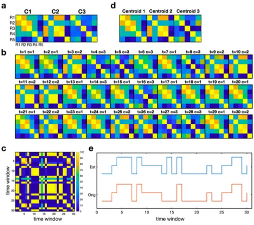
Asanexampleofclusteringforcovariancematrices,wegenerated threetypesofcovariancematriceswithasizeoffive.Wegenerated30 covariancematricesfromthreemodelmatricesC1,C2andC3(10for each).Thethreecovariancematrices(Fig.7a)werederivedfromhuman connectivitymatricesobtainedfromrestingstatefMRI,whichare mu-tuallydistantfromeachotherbasedonalldistancesunderEuclidean, AIRM,andLERMgeometries

𝐶1= ⎡ ⎢ ⎢ ⎢ ⎢ ⎢ ⎣ 1.0000 0.6409 0.2196 0.1736 −0.1886 0.6409 1.0000 0.7230 0.1348 −0.6583 0.2196 0.7230 1.0000 0.2734 −0.6156 0.1736 0.1348 0.2734 1.0000 −0.1824 −0.1886 −0.6583 −0.6156 −0.1824 1.0000 ⎤ ⎥ ⎥ ⎥ ⎥ ⎥ ⎦ 𝐶2= ⎡ ⎢ ⎢ ⎢ ⎢ ⎢ ⎣ 1.0000 −0.0015 0.7898 0.7135 −0.3713 −0.0015 1.0000 0.2193 0.2861 0.1240 0.7898 0.2193 1.0000 0.8958 −0.3887 0.7135 0.2861 0.8958 1.0000 −0.4185 −0.3713 0.1240 −0.3887 −0.4185 1.0000 ⎤ ⎥ ⎥ ⎥ ⎥ ⎥ ⎦ 𝐶3= ⎡ ⎢ ⎢ ⎢ ⎢ ⎢ ⎣ 1.0000 0.5027 0.1763 0.2011 0.4440 0.5027 1.0000 0.0052 0.2146 0.6810 0.1763 0.0052 1.0000 −0.0690 −0.0401 0.2011 0.2146 −0.0690 1.0000 0.3426 0.4440 0.6810 −0.0401 0.3426 1.0000 ⎤ ⎥ ⎥ ⎥ ⎥ ⎥ ⎦

WethenaddedazeromeanGaussiannoisematrixtoeach covari-ancematrixafterweightingitby0.15.Thegeneratedcovariance matri-cesareshowninFig.7b.Forthe30covariancematrices,weexecuted 100k-meansclusteringwithk=3andconstructedafrequency adja-cencymatrix(Fig.7c).Fromthefrequencyadjacencymatrix, modular-ityoptimizationidentifiesthreemodulesandtheirclusterindices.We extractedclustercentroidsforeachclusterbytakinggeodesicaverage ofallmembersforeachcluster(Fig.7d).

3.3. Simulation3.Dynamicconnectivityandstatetransitionanalysis

Asanextension oftheclusteringexample,we conducteda state-transition analysis of functionalconnectivity dynamics (Allenet al., 2014;Damarajuetal.,2014)ontheSPDmanifold.Foragiven tran-sitionmatrix,wesimulatedastatesequence(length=30)consistingof threeheterogeneousstateswhichcorrespondtoinitialcovariance ma-trices,C1,C2andC3(Fig.8a).Thetransitionmatrixusedis

𝑇= ⎡ ⎢ ⎢ ⎣ 9 2 3 4 4 1 2 2 2 ⎤ ⎥ ⎥ ⎦

Forthe30correlationmatrices(Fig.8b),weconducteda modularity-optimization ofmultiplek-meansclustering.Themethodgeneratesa Fig. 7. An example for clustering covariance matri- ces. Three initial covariance matrices (a) were used to generate 30 random variation of covariance matrices around initial covariance matrices (10 for each C1, C2, and C3) (b). (c) displays the frequency adjacency ma- trix of the 30 covariance matrices used for modular- ity optimization. The frequency adjacency matrix indi- cates the frequency for each pair of covariances being a same cluster after 100 repeated k-means clustering. (d) displays the centroids for the three covariance groups.

Fig. 8. State transition analysis of dynamic connectiv- ity. Based on three main correlation matrices C1, C2 and C3 (a), total 30 covariance samples were gener- ated according to a state transition sequence (b). The modularity-based k-means clustering was done after composing a frequency adjacency matrix (c) for 100 it- erations of k-means clustering. The resulting centroids are displayed in (d) and the sequences of original (red) and estimated (blue) ones are displayed in (e) (For in- terpretation of the references to color in this figure leg- end, the reader is referred to the web version of this article.).

frequencyadjacencymatrixbyapplying100repetitionsofk-means clus-tering(Fig.8c),whichwasusedformodularityoptimization.Thecluster centroidsaredisplayedinFig.8dandtheinitialsequenceandresulting sequencearedisplayedinFig.8e.

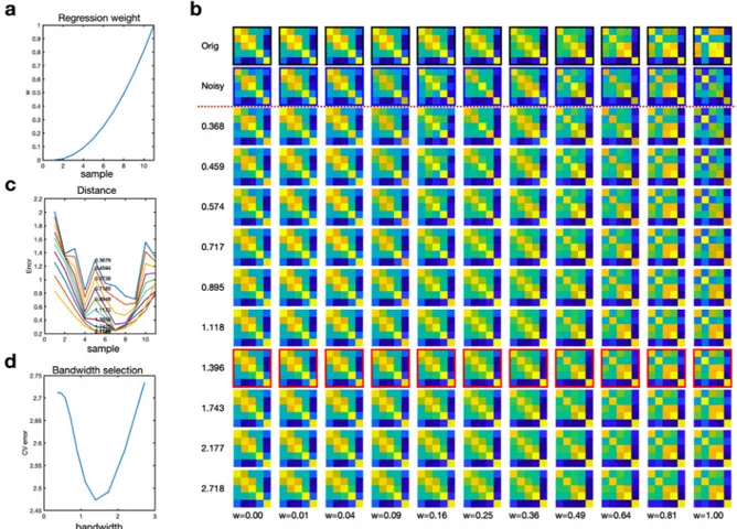
3.4. Simulation4.Smoothingandregression

Weconductedsmoothingofsimulatednoisycovariance matrices. Covariancematricessimulatedweregeometricallypositionedbetween thetwocovariancematricesC1andC2withanexponentially increas-ingdistanceweightw(w=t2 _{fort=[0,0.1,0.2,…,1])forC2and}

1-wforC1onthetangentplane(Fig.9a).Wethenaddedazeromean Gaussiannoisematrixtoeachcovariancematrixafterweightingitby 0.1andprojectedthenoisycovariancematricesbackontothemanifold tomakethemasperturbedobservationsalongthegeodesic.The gen-eratedcovariancesandtheirnoisymatricesareshowninFig.9b.We conducted5-foldcross-validationtodeterminethekernelbandwidthh

fromanexponentiallyequi-spacedintervaloflength10fromexp(-1)to exp(1).Foreachlevelofh,weappliedsmoothingfunctiontothenoisy covariancematrices.Theresultsforsmoothingandbandwidthselection arepresentedinFig.9band9d.

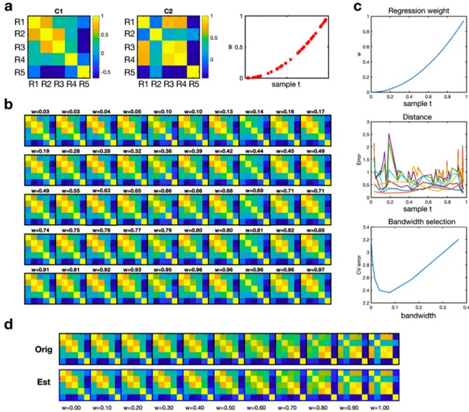
Weutilized this approach toa regressionproblem (Fig.10). We squared 50uniformly distributedweightsandusedthem as interpo-lationweightswforgeometriclocationsbetweenthetwocovariance matricesC1andC2.WethenaddedaGaussiannoiseinthetangent spaceandprojectednoisymatricestosufficeSPDcondition.Usingthe bandwidthhcorrespondingtotheminimalk-foldcross-validationerror, weestimatedaninterpolationfunction,whichpredictsthecovariance matrixatanygeometriclocation(correspondingtoaweightw).

3.5. Simulation5.Principalgeodesicanalysis

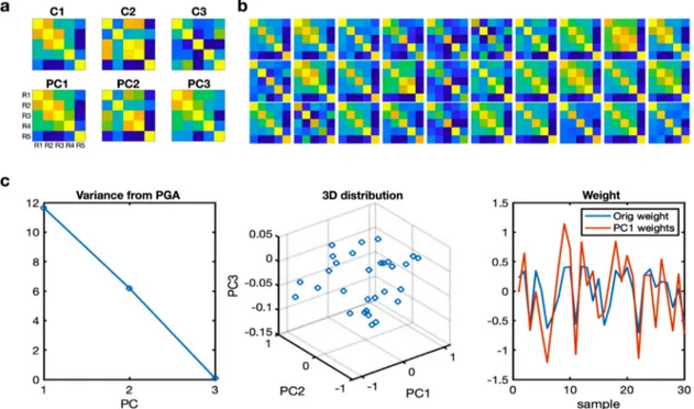
Wegenerated30covariancesamplesbyinterpolatingthreetarget co-variances(C1,C2andC3)withrandomweights(Fig.11a).Theweights werederivedfromauniformdistributionbuttheweightsforC1were

multipliedby1.2fromtheinitialweightstoemphasize variationsof C1.Theweightedsumwasdoneinthetangentialspace.Theresult co-variancesamplesarepresentedinFig.11b.Wethenappliedprincipal geodesicanalysistothecovariancematricestofindprincipalgeodesics andtheirweightsforthesamples(Fig.11c).

3.6. Simulation6.Testofequaldistributions

In statistical literature of hypothesis testing, simulation study is often adopted to demonstrate the power of a proposed procedure (LehmannandRomano,2010).Amongseveralindices,wereport empir-icaltype1error,whichmeasuresratiooffalserejectionswhenthenull hypothesisof𝐻0∶𝐹𝑥=𝐹𝑦istrue.Inoursimulation,weusetwo

exem-plarytestswithsamplesdrawnfromthecorrelationmatricesC2andC3. Foreachgroup,wegeneratetimeseriessamplesfromWishart distribu-tionbyusingdesignatedcorrelationmatrixasascaleparameterand𝜈

degreesoffreedom(timeserieslength)andnormalizethematricesto haveunitdiagonals.Weused𝜈 =50toguaranteestrictpositive definite-ness.Wevariedthenumberofobservations(correspondingtosubjects inthegroupstudy)belongingtoeachsetfromn=5to50inorderto checkanimpactofsamplesizeontheperformance.ForT=500 iter-ations,twosetsofcorrelationmatriceswithvaryingsamplesizesfrom

n=5to50arerandomlygeneratedinaccordancewiththeprocedure describedaboveandp-valuesarerecorded.Then,empiricaltype1error atthepre-definedsignificancelevel𝛼 isobtainedby

Type1Error=#{𝑐𝑜𝑚𝑝𝑢𝑡𝑒𝑑𝑝-𝑣𝑎𝑙𝑢𝑒𝑠 ≤ 𝛼}

𝑇

andweconcludethetestisvalidifempiricaltype1errorissimilarto𝛼.

AsshowninFig.12,bothexamplesshowsimilarlevelsoftype1errors and𝛼 =0.05fordifferentnumbersofobservations.

3.7. Experimentaldataanalysis

Fortheexperimentaldataanalysis,weused734rs-fMRIdata(2016 release,male:N=328,female:N=405,age:22~37,mean:28.7,std:3.7)

Fig. 9. An example for smoothing of continuously varying correlation matrices with Gaussian noises. A set of noisy continuous covariance matrices (the first row in (b)) were generated by weighted summing of two covariance matrices (C1 and C2 in Fig.7) with a Gaussian noise in the tangent plane. The weight is presented in (a). For ten different bandwidths, the distances between samples and their corresponding regressed ones are presented in (c). The 5-fold cross validation (CV) errors for all bandwidths are presented in (d). The original covariance samples are displayed in the first row and their noisy versions are displayed in the second row of (b). The lowest CV error was found at the bandwidth of 1.396, the 9th row in (b).

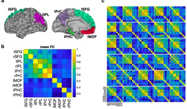
fromtheHumanConnectomeProject(HCP)database(VanEssenetal., 2012).Alldatawassampledat0.72Hzduringfoursessions,with1200 timepoints per session. rs-fMRI datawas preprocessedaccordingto theHCPminimalpreprocessingpipelineandmappedintocortical sur-faces(Glasseretal.,2013).Fortheanalysisofbrainnetworks,we ex-tractedtimeseriesattenbrainregionsinthecorticalsurface-based at-las(Desikanetal.,2006)correspondingtothedefaultmodenetwork (DMN).Theyarethesuperiorfrontalgyrus(SFG,alsoknownasthe dorsomedialprefrontalcortex),medialorbitofrontalcortex(MOF, cor-respondingtoventromedialprefrontalcortex),parahippocampus(asa partofthehippocampalformation),precuneusandinferiorparietallobe ineachhemisphere(Fig.13A),whicharecommonlyfoundinprevious studiesofDMN (Buckneretal.,2008;Poweretal.,2011;Yeoetal., 2011).Thefirsteigenvariatederivedfromtheprincipalcomponent anal-ysisoffMRItimeseriesatsurfacenodesforeachregionwasusedasa regionalBOLDsignalsummaryfortheregion.Pearsoncorrelationof rs-fMRIwasusedasameasureforfunctionalconnectivityofthetime series.Thegeodesicaverageofallthe734rs-fMRIdataandexemplary functionalconnectivity(correlation) matricesof 30subjects are pre-sentedinFig.13band13c.

3.8. Experiment1.Regressionanalysis

We conducted a regression analysis of connectivity matrices ac- cording to behavior scores. Among many behavior scores in the HCP database, we chose Penn Matrix Test (PMAT) and Pittsburgh Sleep Quality Index (PSQI) to test the feasibility of geodesic re- gression analysis for SPD. The PMAT24 which was developed by

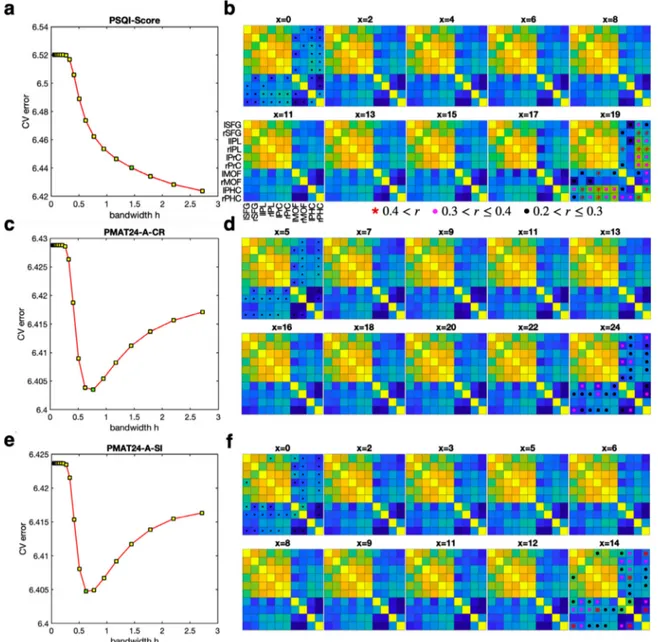
Gur and colleagues ( Bilker et al., 2012) is a shortened version of the Raven’s Progressive Matrices that measures fluid intelli- gence. To represent fluid intelligence, number of correct responses (PMAT24_A_CR) and total skipped items (PMAT24_A_SI) were used. The PSQI test is a widely used 19 self-rated questionnaire that as- sesses sleep quality and disturbances over one month time inter- val ( Buysseetal., 1989). In the SPD regression analysis, we de- termined the kernel bandwidth by utilizing 5-fold cross valida- tion at 20 exponentially equidistant bandwidths ( Fig.14a, c and e). With the kernel bandwidth showing minimal CV errors (for concave CV-error curves, e.g., PMAT24-A-CR and PMAT24-A-SI) or knee of CV-error curves (for curves without any local minima, e.g., PSQI-scores), 734 connectivity matrices at different scores for each measure were used to estimate regression function. The represen- tative connectivity matrix at each score according to the learned regression function is presented in Fig.14b, d and f.

3.9. Experiment2.Principalgeodesicanalysis(PGA)

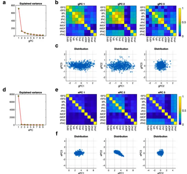
Principalgeodesicanalysiswasappliedtothe734connectivity ma-trices,fromwhich nineprincipalgeodesiccomponentswerederived. Theexplainedvariancesofallninecomponentsandtopthreeprincipal geodesiccomponentsandtheircoefficients(theweightofconnectivity matricesprojectedontoeachcomponent)aredisplayedinFig.15a–c. Thecomponent3differsfromtheothercomponentsinthatthe mod-ulecomposedofthebilateralinferiorparietallobeandtheprecuneus aredifferentiatedfrom otherbrainregions.Thecomponent2differs fromthecomponent1intheisolatedmedialorbitofrontalcortex.The

Fig. 10. An example for regression analysis of covariance samples. By weighted summation of C1 and C2 covariance matrices (a) using a square weighted function w (the third panel of a), followed by adding Gaussian noise, we generated 30 samples of correlation matrices (b). The evaluation of regression performance was done at the weight points shown in (c). For ten different bandwidths, the distances between samples and their corresponding regressed ones are presented in the middle panel of (c). The 5-fold cross validation (CV) error for each bandwidth is presented in the bottom panel of (c). The original covariance samples and regressed correlation matrices (with an optimal bandwidth) at ten uniformly spaced weight points are displayed in (d).

geodesiccomponent1explainsmostportionsofvariabilityof connec-tivitymatricesasshowninthedistributionofcoefficients(Fig.15c). WealsoevaluatedEuclideanprincipalcomponentanalysisforthe co-variancematricesasasetofvectors(onepereachsubject)without con-sideringcovariancearchitecture.TheresultsarepresentedinFig.15d–f. ThedistributionsofcomponentsandtheircoefficientsintheEuclidean analysisdifferfromthoseofgeodesicanalysis.

3.10. Experiment3.Clustering

Modularity-optimizationofmultiplek-meansclusteringwasapplied to734connectivitymatrices.Atotalof100runsofk-meansclustering constitutesafrequencyadjacencymatrix(Fig.16a),whichwassorted bymodularityoptimization(Fig.16b).Thefrequencyadjacencymatrix indicateshowmucheachpairofnodesisassignedtoasameclusterfor partitionsfromk-meansclustering.Connectivitymatricesof734 sub-jectsarecategorizedintothreeclustersaccordingtothisapproach.The geodesicmeanandEuclideanmeanforeachclusterandtheirdifference arepresentedinFig.16c-e.Theclustercenters1,2,and3matchhighly withgeodesicprincipalcomponents1,3and2inFig.15.

3.11. Experiment4.Dynamicconnectivity

Dynamicsinthefunctionalconnectivitywasevaluatedbyclustering sliding-windowedconnectivitymatrices,followedbycalculatinga tran-sitionmatrixamongtheclusters.rs-fMRItimeseriesdata(1200 tempo-ralscans)fromasubjectwasdividedinto83epochsbyaslidingwindow approachwithawindowsizeof42(30s,0.72sec/sample)andan over-lapof28 (20s)(Fig.17a).Wecalculatedcorrelationmatricesforall theepochs.Total100k-meansclusteringwereappliedtothe83 corre-lationmatricesintheSPDspacetocomposeafrequencyadjacency ma-trix(Fig.17b),whichwasusedformodularityoptimization(Fig.17c). Wepresentedthethreegeodesicclustercenters(Fig.17d)andthe tran-sitionmatrixthatshowsthenumberoftransitionsamongtheclusters (Fig.17e).

3.12. Experiment5.PerformancecomparisonbetweenAIRMandLERM

We presented thereliabilityand computationalburden innate to intrinsicFréchetmeancomputationusingAIRMagainstlog-Euclidean counterpart(LERM)inFig.18.Itiscommonpracticetotakeextrinsic

Fig. 11. An example for principal geodesic analysis (PGA) of correlation matrices. 30 correlation matrices in (b) were generated by randomly weighting C1, C2 and C3 correlation matrices in (a). The weights for C1 were multiplied by 1.2. The explained variances of principal components are displayed in the first panel of (c). The sample distributions in the principal component axes are shown in the second panel of (c). The initial weights for C1 and weights for the first principal component (PC1) are displayed in the third panel of (c).

meanasastartingpointforgradientdescentalgorithmduetoits asymp-toticconvergence(BhattacharyaandBhattacharya,2012).Thismeans thatthestrategywetakeinevitablyrequiresadditionalcomputingtime foraniterativeschemebutitmaybenegligiblysmallbytakingagood starting point. Wecompare theperformance of twoaforementioned frameworksin computingFréchet meanof1000covariancematrices Σ_𝑖,𝑖=1,…,1000 independently generated from Wishart distribution

𝑊𝑝(𝑉,𝑛)forarangeofdimensions(networksize)𝑝=50, 100,…,500,

𝑉 =𝐼_𝑝ascalematrixwith𝑛=10000 degreesoffreedomwhichis suf-ficienttoguaranteethedefinitenessof generatedsamples.Themean squareddifferencebetweenmeancovariancesestimatedbyusingAIRM andLERMis presentedin theleft panelofFig.18 andtheCPUtime insecondsaredisplayedintherightpanelofFig.18.Theexperiment wasconductedonapersonalcomputerwithaquad-coreInteli7CPU

runningat4GHzand24GBRAM(AppleiMac,2014)usingMATLAB R2019bwithoutanyexplicitparallelcomputinginvolved.

4. Discussion

Useofcorrelationmatrixforrestingstateortask-dependentfMRIhas beenabasictoolforfunctionalbrainnetworkanalysis.Theimplicit as-sumptionofconventionalfunctionalnetworkanalysisisthateachedge isconstructed(andcanbedealtwith)separatelyfromotheredgesby repetitivepairwisecorrelationanalysis.Ithaslittleconsideredthe cor-relationmatrixasawholeandoftenneglectscorrelatednatureofedges. Insomeapplications,multipleedgesaremodeledtobejointlyinvolved in thebraindiseases orcognitions.However,thevectorization-based multivariateapproachdoesnotacknowledgethateachedgeitselfisa

Fig. 12. Test of equal distributions. (a) and (b) show empirical type 1 errors with increasing number of observations in the x-axis for simulations with C2 and C3 at the significance level 𝛼 =0 .05 .

Fig. 13. The brain regions used in the evaluation of the default mode network. a) The brain network includes the superior frontal gyrus (SFG), medial orbitofrontal cortex (MOF), parahippocampus (PHC), precuneus (PrC) and inferior parietal lobe (IPL) according to the Desikan-Killiany atlas ( Desikanetal.,2006). The brain regions in the left hemisphere are presented. The first letters “l ” and “r ” in each region’s name indicate left and right hemisphere. b) The geometric average of a group of 734 functional connectivity matrices (FC) is presented. All square pixels in the connectivity matrix indicate edges among the brain regions. Dots in (b) indicate edges that show 5% differences between Euclidean average and geometric average of group connectivity matrices. c) Functional connectivity matrices of 30 exemplary subjects are displayed.

resultofmulti-nodalactivitiesandhasinterrelatednesswithothersin consequence.Itisnotdifficulttofindneurobiologicalexamplesthatthe basicassumptiondoesnothold.Forexample,somenodes(suchasthe ventraltegmentalareaandthesubstantianigraparscompactainthe dopaminepathwayortheraphenucleusintheserotoninpathway)play modulatoryrolesformultipleedges(thus,theyareinterrelated). There-fore,asingleedgemaywellbe consideredin associationwithother edges.Thisistherationaletodealwithcorrelationmatrixasawhole.

SincethecorrelationmatrixisatypeofSPDobjectswhichhavea cone-shapeRiemanniangeometry,weneedtotakeadvantageofdealing correlationmatricesasmanifold-valuedobjectswithcorresponding ge-ometricstructure.Persistentinversionofcovariancematricesforgroups inFigs.5 and6 issuchanexample.Wecanalsofindseveralexamples onthefunctionalconnectivityanalysisusingthecorrelationmatrixon theSPDmanifold(Daietal.,2016;Daietal.,2020;Deligiannietal., 2011;Ginestetetal.,2017;Ngetal.,2016;Qiuetal.,2015;Rahimetal., 2019;Varoquauxetal.,2010;Yaminetal.,2019).

Varoquauxetal.(2010) introducedFréchetmeanandvariationof correlationmatricestodetectfunctionalconnectivitydifferenceinthe post-strokepatientsusinggroup-levelcovarianceaveragesand demon-stratedanincreasedstatisticalpowerinthedetectioncomparedtothe Euclideanspace.Theyalsoproposedabootstrapprocedureforpairwise coefficientanalysisonthetangentspacetoensuremutualindependence amidcoordinates.Incomparedtotheirstudy,wepropose bootstrap-pingdirectlyonintra-groupdifferencestoinferstatisticalsignificance ofedgedifference.Rahimetal.(2019) utilizedSPDgeometryin esti-matingfunctionalconnectivityofindividualsbypullingallcovariance matricestotangentspacearoundFréchetmeanandconstructedan em-piricalpriorderivedfromthetangentializeddatatobeusedasa group-levelshrinkagemechanismforindividualcovariances.Inestimating be-haviorsusingcovariancematrix,Ngetal.(2016) utilizedawhitening transportapproachwhichapplieslogmappingalongtheidentitymatrix afterremovingthereferencecovarianceeffectinsteadofconventional paralleltransportapproach.Ginestetetal.(2017) proposedamethod tohypothesistestingforbinarizedconnectivitymatrixintheSPDspace

usingthegraphLaplacianmatrixwhichinheritsSPDstructurebyits na-ture.Yaminetal.(2019)comparedbrainnetworksbetweentwinswith geodesicdistanceontheSPDmanifold.Deligiannietal.(2011)proposed aregressionanalysisontheSPDmanifoldininferringbrainfunctional connectivityfromanatomicalconnections.Thechangepointdetection hasalsobeenconductedintheSPDspacebyDaietal.(2016)who con-ductedstationaritytestingof functionalconnectivityobtained bythe minimalspanningtreeinconjunctionwithresampling-baseddecision rules.Daietal.(2020)alsoproposedametricfortrajectoriesontheSPD manifoldtolearnindividuals’dynamicalfunctionalconnectivityatthe populationlevelbasedondistance-basedlearningmethods.Thismainly differsfromcurrentsmoothingapproachproposedbyLinetal.,(2017) inthatwestandinlineforanonparametricmodelingofthesmoothed trajectory itself. BesidesfMRI study, Sadatnejad et al. (2019) intro-ducedaclusteringmethodontheSPDtorepresentEEG.Severalstudies haveconducteddimensionreductionformachinelearningintheSPD space.Qiu etal.(2015) conductedamanifoldlearningonfunctional networks usingregressionuponageaftertransforming covarianceto theEuclideanspacebyapplyinglogarithmicmapattheidentity ma-trix.Davoudietal.(2017) suggestedadimensionalityreductionbased ondistancepreservationtolocalmeanforsymmetricpositivedefinite matrices.Xieetal.(2017)alsoconductedclassificationafterdimension reductionbasedonbilinearsub-manifoldlearningofSPD.

The current studycan be in linewithandan extension ofthose previousstudies,byintroducingmorealgorithmsinparticularto func-tionalbrainnetworkanalysis,whichwerepreviouslyusedor concep-tualizedintheSPDresearchfields.Theinferencealgorithmswenewly introducedinthefunctionalconnectivityanalysisaresmoothingand re-gression,principalgeodesicanalysis,clusteringandstatisticaltestsfor correlation-basedfunctionalconnectivity.

TheregressionofSPDistofindarelationshipbetweenacovariate andcovariancematrix,whichwasgenerallyapproximatedby minimiz-ingerrors(measureddataminuspredictedoneswithalearned regres-sionfunction).ThisregressionframeworkforSPDisnottrivialsincethe conceptofsubtractionmaynotbestraightforward.Linetal.(2017)

pro-Fig. 14. Geodesic regression analyses for connectivity matrices with Pittsburgh Sleep Quality Index (PSQI) score (a and b), Number of Correct Responses of Penn Progressive Matrices (PMAT24_A_CR) (c and d) and Total Skipped Items of Penn Progressive Matrices (PMAT24_A_SI) (e and f). To optimize the regression kernel bandwidth, 5-folds cross-validation (CV) errors were calculated for every bandwidths h (a, c and e). The bandwidths were set to be exponentially increasing from exp(-3) to exp(1) in 20 steps. The bandwidth that have minimal CV errors or curve knee points were chosen to be optimal (green rectangle). The regression results were presented in the form of connectivity matrix for a 10 equispaced scores (x) from the minimum to the maximum scores (b, d and f). To designate changes in the edges for visualization purpose, we marked edges that have 20%, 30% and 40% change ratios between the connectivity matrices of the lowest (the regressed connectivity for the first score, C 1) and highest scores (the regressed connectivity for the last score, C n). The ratio r was defined by the absolute difference between the

connectivity for the first and last scores, normalized by the mean connectivity across all scores, 𝑟= |𝐶𝑛−𝐶1| 1 𝑁

∑𝑛

𝑖=1𝐶𝑖× 100 , where C iindicates the representative (regressed)

connectivity matrix at the score i (For interpretation of the references to color in this figure legend, the reader is referred to the web version of this article.).

poseda powerful regressionmethod associating manifold-valued re-sponseandvector-valuedexplanatoryvariablesbyapplyingkernel re-gressionontotransformedresponsesundersomeembeddingthat pre-servesgeometricinformation(Nadaraya,1964;Watson,1964).We uti-lizedthisnonparametricregressionframeworktoassociatefunctional connectivityagainstone-dimensionalcovariate.Althoughwe focused onaone-dimensionalcovariateforsimplicityinthecurrentstudy,this regressioncan be easily extendedto caseswith multiple covariates. Thisapproachdiffersfrommostofpreviousstudiesonregression anal-ysisoffunctionalnetworks,whichhavedealtwithcorrelation matri-ceselement(edge)byelement(edge)separatelyfromeachotheredge (Dosenbachetal.,2010;Siman-Tovetal.,2016).Theintroduced regres-sionalsodiffersfromQiuetal.(2015) whichperformsLocallyLinear

Embeddingtoembedmanifold-valuedcovariatesintoEuclideanspace sothatconventionalregressionmodelscandirectlybeused.However, themethodbyQiuetal.(2015) doesnotguaranteestraight-forward interpretationofacquiredregressioncoefficients.

IntheSPDsmoothingandregressionanalysis,themainissueishow todeterminethekernelbandwidth(orsmoothness)residingintheSPD data.Sincethecurrentgeodesicsmoothingisadata-drivenapproach, weoptedforacross-validationschemetodeterminethekernel band-width‘h’.Whenweappliedtheproposedregressionanalysisto func-tionalnetworksaccordingtobehaviorscores, i.e.,thePSQIscoresor PMATscores,itestimatesmeaningfularchitectureinthefunctional net-work.TheresultsuggeststheadvantageofSPDregressioninexploring howfunctionalnetworkchangesalongacovariateasawhole,not

ele-Fig. 15. Principal geodesic analysis and Euclidean principal component analysis of connectivity matrices. The explained variance for 9 components is presented in (a). The top three principal geodesic components (gPC) derived from 734 connectivity matrices are presented in (b). The distributions of coefficients for all connectivity matrices projected onto the top three components are presented in (c). Euclidean principal component analysis shows different explained variance curve (d) and components (e) compared to those of geodesic component analysis. Distributions of 734 coefficients for the three principal components, ePC1, ePC2 and ePC3, are displayed in (f).

mentbyelement.Inthecurrentstudy,weevaluatedtheperformanceof thecurrentsmoothingandregressionanalysisforaprespecifiednoise level. Further elaboration witha moreextensive rangeof noise lev-elswillbeworthyinunderstandingtheperformanceoftheproposed method.

Asa multivariateanalysis of covariancematrices, principal com-ponent analysis (Leonardi et al., 2013) or independent component analysis (Park et al., 2014) has been used in the Euclidean space. Fletcher et al. (2004) introduced a principal geodesic analysis onto thesettingwithmanifold-valueddata.Sincethereisnodirect counter-partof empiricalcovariancematrixandeigen-decompositionon Rie-mannian manifold,a local approach was first takenin thestudy of Fletcheretal.(2004).Sofar,theprincipalgeodesicanalysishasbeen appliedtoshapeanalysis(Aljabaretal.,2010;Fletcheretal., 2004) anddiffusiontensoranalysis(FletcherandJoshi,2004).Inthisstudy, weintroduceprincipalgeodesicanalysistotheanalysisoffunctional networksintheformofcorrelationmatrices.AsshowninFig.15,there aresignificantdifferencesintheprincipalcomponentsandtheir coeffi-cientsbetweenthetwoapproaches.Asalimitationinprincipalgeodesic analysisforthenetworkanalysis,notmuchisknownfornoiseeffects (inthecovariancematrix)ontheprincipalgeodesicanalysis.We

can-notdisregardthecomputationalcostforthelarge-sample,large-scale networkanalysis.

k-means,thoughpowerfulintheclustering,isknowntosufferfrom two majordrawbacks.First, itis NP-hardin generalso that finding the optimalsolutionis troublesome (Aloise etal., 2009).Lloyd’s al-gorithmprovidesaheuristicapproachtoobtainsuboptimalsolutions givenaninitializationbutoutcomevariabilitycannotberemovedby differentinitialpartitioning(Celebietal.,2013).Althoughmany vari-antshavebeenproposedtoovercomesuchinstabilityincludinga pop-ularinitializationmethodk-means++(ArthurandVassilvitskii,2007), westillchooserandominitializationschemesinceextracomputational complexitybysuchmethodscanbehighespeciallyinourcontext.Some methodscannotbedirectlytransferredduetoourgeometricrestrictions wherethestructureofEuclideangeometrycannotbedirectly transfer-able.Wecanachievegood-enoughsolutionsviaparallelcomputingon multipleinitializations.Theseconddrawbackofistheselectionof clus-ternumbersk.UnlikeprobabilisticandBayesianmethodswhere statis-ticalinferenceonkisachievablewithintheirmodelingframework,a familyofk-partitioningalgorithms-k-meansanditsvariants– requires posthocmodelselectionprocedurestodeterminethenumberof clus-ters.Amongmanyclusterqualityscores,weimplementanadaptation

Fig. 16. Modularity optimization of multiple k-means clustering. Total 100 runs of k-means clustering compose a frequency adjacency matrix of all pairs of two nodes being in a same cluster (a). The modularity optimization of the frequency adjacency matrix results in sorted clusters (b). The centers for all three clusters derived by geodesic mean (c), Euclidean mean (d) and their difference (e) are presented.

ofcelebratedSilhouettemethod(Rousseeuw,1987)toourcontextsince itonlyreliesonanydistancemetric.

Toovercometheproblemsinherentinthek-meansclusteringsuch asdependencyontheinitialvalueandcluster number,wegrafteda modularity-basedclusteringmethod(Jungetal.,2019)ontoSPDspace. Thisclusteringapproachconstructsafrequencyadjacencymatrixthat countspartitionco-occurrenceforeachpairofsamplesaftermultiple runs of k-means clustering. The modularityoptimization of the fre-quencyadjacencymatrixleadstoreliableclusteringofcorrelation ma-trices,robusttoselectionofinitialvaluesandclusternumbers.

Tonote,ClusterValidityIndexisathematicprogramtomeasure ef-fectivenessofagivenclusteringthoughithasnotbeenfullyextended forRiemannianmanifold.Theextensionofthepopularevaluation in-dicesfromliteraturetolarge-scaleclusteringoffunctionalconnectivity matricesremainstoberesearchedfurther.

AnySPDclusteringalgorithmscanreadilybeusedtotheanalysisof dynamicfunctionalnetworksasshowninFig.17.Thedynamicsof func-tionalconnectivityhasbeensummarized bytransitionmatrixamong severalrepresentativestates,whichwasestimatedbyk-means cluster-ingintheEuclideanspace(Allenetal.,2014;Damarajuetal.,2014). Weshowedthatthisframeworkfordynamicconnectivityanalysiscan beappliedintheSPDspace.

Asmentionedearlier,acollectionofcorrelationmatricestakes ac-countintoa submanifoldof SPD matriceswitha unitdiagonal con-straint.Thiscausessomeoperationswithcorrelationmatricesnot neces-sarilyresultinginanothercorrelationmatrix.Inthisstudy,we normal-izedresultingmatricesintocorrelationmatriceswhenevernecessary un-derthephilosophyofiterativeprojectionontothesubmanifold,which isaconstrainedsetwithinSPDmanifold.Ifweconsideroneconvention tonormalizeBOLDsignalstoruleouttheeffectofsignals’magnitude, thisinevitablyconvertscovariancetocorrelationmatriceswhilethe lit-eraturehasbeenlittlecarefulindistinguishingunexpectedimpactof suchscenario.Atthisstage,weresorttoanad-hocapproachtodeal withcorrelationmatricesevenwithintheSPDgeometricstructure.One

candidatetoovercomesuchinconvenienceincludeselliptopestructure eventhoughcurrentliteraturelargelydealswithrank-deficient correla-tionmatrixandlacksconcretetheoreticalstudiesatthemoment.Forthe full-rankscenario,itispossibletoconsideraRiemanniansubmersionby anisometricactionbythesetofpositivediagonalmatricesfromtheLie grouptheorytoextendtheaffine-invariantframework.However,this exponentiatesthecomputationalburdenwhilethegainisthincompared tothatofourad-hocapproach.Thisnecessitatestofurtherextensive in-vestigationofwhatwewouldbenefitfromadoptingsuchstructure.

Statisticalanalysisorclassificationoffunctionalconnectivityover theSPDmanifoldisrecommendedcomparedtodirectlyapplyingthose methodstovectorizedcorrelationmatricesbecausetheinter-relatedness amongelementsinthecovariancematricesviolates“theuncorrelated featureassumption” implicitinmoststatisticalanalysisorclassification algorithms(Ngetal.,2016).Inpractice,however,analysisoffunctional connectivityunderSPDframeworkmaynotalwaysbebeneficial com-paredtotheEuclideantreatmentinstatisticalanalysisorinthemachine learning. Thismaybe particularlytrue in thehighdimensional net-workswhichincurshighcomputationalcost.Onepossiblebottleneck comesfromanobservationthatinbothAIRMandLERMgeometries,an atomicoperationthatisnomorealgorithmicallydivisibleinvolves ma-trixexponentialandlogarithmwhichareofcomparablecomplexityas eigen-decompositionofsymmetricmatrices.Still,itdoesnotnecessarily hamperapplicationofgeometricapproachesaslongasoneavoids anal-ysisatthescalelargerthantensofthousandsofvariableswithmodern computingcapabilities.Althoughthisisnotusualinthegeneral neu-roimagingresearches(mostlylessthan500ROIs– ittakesabout300s tocalculategeometricmeanof1000covariancesmatriceswithasizeof 500asshowninFig.18),executingaforementionedoperationsrequires heavyexploitationofcomputinghardware,efficientdesignofmemory use,andspecializedlibrariesdesignedforscalablecomputation,which isaninterestingresearchdirectionofitsownimportanceinthefuture. Wewouldalsoliketopointoutonerequirementforapplicationof theintroducedframework.Whenthenumberofscansissmallornot

Fig. 17. State transition analysis of dynamic functional connectivity. A rs-fMRI time series of 1200 samples was divided into 83 consecutive epochs (a window size of 42 samples with 28 samples of overlap) (a) and correlation matrices were calculated from each epoch. The vertical lines indicate the starting point of each epoch (the gap is 28 samples). The 83 correlation matrices were clustered into three clusters using the modularization optimization of frequency adjacency matrix (b) from 100 runs of k-means clustering. The sorted frequency adjacency matrix is presented in (c). The centers for the three modules were evaluated by geodesic average of the connectivity matrices of the three modules (d). The state transition matrix among the three states (connectivity matrix) is presented in (e).

Fig. 18. Comparison between AIRM and LERM. The mean squared difference between Fréchet mean of 1000 generated covariances estimated by using AIRM and LERM with different matrix sizes (left) and the average computational time (in seconds) to compute Fréchet mean of 1000 covariance matrices with different matrix sizes (right).