http://osj.kr
Influence of Seasonal Forcing on Habitat Use by Bottlenose Dolphins
Tursiops truncatus in the Northern Adriatic Sea
Giovanni Bearzi
1*, Arianna Azzellino
1,2, Elena Politi
1, Marina Costa
1, and Mauro Bastianini
1,31Tethys Research Institute, Viale G.B. Gadio 2, 20121 Milan, Italy
2Politecnico di Milano, DIIAR Environmental Engineering Dept, P.zza Leonardo da Vinci 32, 20133 Milan, Italy 3CNR-ISMAR, Istituto di Scienze Marine, Castello 1364/A, 30122 Venice, Italy
Received 17 June 2008; Revised 20 September 2008; Accepted 5 December 2008
Abstract − Bottlenose dolphins are the only cetaceans regularly observed in the northern Adriatic Sea, but they survive at low densities and are exposed to significant threats. This study investigates some of the factors that influence habitat use by the animals in a largely homogeneous environment by combining dolphin data with hydrological and physiographical variables sampled from oceanographic ships. Surveys were conducted year-round between 2003 and 2006, totalling 3,397 km of effort. Habitat modelling based on a binary stepwise logistic regression analysis predicted between 81% and 93% of the cells where animals were present. Seven environmental covariates were important predictors: oxygen saturation, water temperature, density anomaly, gradient of density anomaly, turbidity, distance from the nearest coast and bottom depth. The model selected consistent predictors in spring and summer. However, the relationship (inverse or direct) between each predictor and dolphin presence varied among seasons, and different predictors were selected in fall. This suggests that dolphin distribution changed depending on seasonal forcing. As the study area is relatively uniform in terms of bottom topography, habitat use by the animals seems to depend on complex interactions among hydrological variables, caused primarily by seasonal change and likely to determine shifts in prey distribution.
Key words − common bottlenose dolphin, Tursiops truncatus, habitat use, Adriatic Sea, Mediterranean Sea
1. Introduction
The northern Adriatic Sea is one of the few Mediterranean areas with historical information on cetaceans (Bearzi et al. 2008b). Two cetacean species have been consistently
abundant there until recent times: the short-beaked common dolphin Delphinus delphis and the common bottlenose dolphin Tursiops truncatus (hereafter bottlenose dolphin). Intentional killings and systematic dolphin extermination campaigns conducted for over a century as an attempt to reduce conflict with fisheries caused significant dolphin mortality until the 1960s (possibly several thousands of animals; Bearzi et al. 2004). Unsustainable killings are thought to have triggered the decline of short-beaked common dolphins. In addition, habitat degradation and changes in prey availability in subsequent years probably accelerated the decline of this species. Bottlenose dolphins are also likely to have suffered from intentional killings in historical times, followed by ongoing habitat degradation and prey depletion caused by excessive fishing. Today, bottlenose dolphins remain the only cetaceans regularly observed in the northern Adriatic, but they survive at relatively low densities compared to other Mediterranean areas (Bearzi et al. 2000, 2004).
In such a scenario, monitoring dolphin populations and understanding their patterns of distribution and the factors influencing their habitat selection is critical for developing management and conservation plans and for complying to a commitment of ensuring a ‘favourable conservation status’ to cetacean populations in the Mediterranean. This commitment has been expressed by a large number of international agreements (see review in Bearzi et al. 2008b), including the European Union ‘Habitats Directive’ and the ‘Convention on the Conservation of Migratory Species of Wild Animals’ by the United Nations Environment Programme.
*Corresponding author. E-mail: [email protected]
Because field research on Adriatic cetaceans has been scant and restricted to a few local areas where resident coastal communities of bottlenose dolphins have been studied intensively (e.g. in the Kvarneric, Bearzi et al. 1997, 1999; Fortuna 2006), little is known about their ecology and habitat use. This study is one of the most extensive investigations on cetaceans in inshore and offshore Adriatic waters, and aims to disclose some of the factors that determine habitat use by bottlenose dolphins in a topographically-homogeneous environment.
While habitat preferences of dolphins may be influenced primarily by the distribution of their prey, several studies have suggested the possibility of defining habitat selection by delphinid species around the world in terms of physiography and hydrography. Various relationships between the distribution of cetaceans and oceanographic features have been demonstrated for small Delphinidae including Delphinus sp. (Evans 1975; Hui 1979, 1985; Polacheck 1987; Selzer and Payne 1988; Reilly 1990; Silber et al. 1994; Fiedler et al. 1998; Goold 1998; Hooker et al. 1999; Cañadas et al. 2002; Ferguson et al. 2006), Stenella sp. (Polacheck 1987; Reilly 1990; Mullin et al. 1994; Hooker et al. 1999; Cañadas et al. 2002; Davis et al. 2002; Griffin and Griffin 2003; Ferguson et al. 2006; Azzellino et al. 2008), Lagenorhynchus sp. (Selzer and Payne 1988; Hooker et al. 1999; Yen et al. 2004; Tynan et al. 2005), Hector’s dolphins Cephalorhynchus hectori (Bräger et al. 2003), Fraser’s dolphins Lagenodelphis hosei (Davis et al. 2002), rough-toothed dolphins Steno bredanensis (Davis et al. 2002; Ferguson et al. 2006), Risso’s dolphins Grampus griseus (Polacheck 1987; Mullin et al. 1994; Baumgartner 1997; Cañadas et al. 2002; Davis et al. 2002; Yen et al. 2004; Ferguson et al. 2006; Azzellino et al. 2008), and bottlenose dolphins (Polacheck 1987; Mullin et al. 1994; Silber et al. 1994; Hooker et al. 1999; Cañadas et al. 2002, 2005; Davis et al. 2002; Griffin and Griffin 2003; Ferguson et al. 2006).
Most cetacean species have been shown to display relatively consistent preferences in terms of bottom topography and water depth, including in the Mediterranean Sea (Azzellino et al. 2008). However, the relationships between dolphin habitat preferences and hydrological variables have been investigated less often and results have varied among species and areas. Hydrological features are thought to affect the distribution and density of cetacean prey through mechanisms such as concentration of nutrients, increased primary production, or aggregation of biomass due to
convergence of water masses (Cañadas et al. 2002; Davis et al. 2002).
The possibility of investigating the influence of hydrological variables is often limited by the difficulty of combining cetacean surveys with systematic measurements of these variables. This work has benefited from the opportunity of conducting dolphin observations in parallel with hydrologic research, with the resulting possibility of combining effort-weighted dolphin data with 1) physiographical variables (bottom depth and distance from the nearest coast), and 2) a wide array of hydrological variables recorded in different seasons.
2. Materials and Methods
The study area encompasses the north-western portion of the Adriatic Sea delimited by the Italian coast to the north and west, and by waters up to 44°32’N and 13°31’E (Fig. 1). This area covers approximately 8,500 km2 of sea surface. The sea floor is less than 50 m deep and consistently sandy or muddy. The study area is characterized by high interannual and seasonal variability of hydrological and biological variables (Zavatarelli et al. 1998). Water clarity is highly variable (for instance, Secchi disk values recorded during the study period ranged between 0.5 and 23.5 m). Interactions between the Po river flow and the seasonal dynamics of the Adriatic circulation and thermal cycle determine a highly variable distribution of nutrients (Socal et al. 2002) that combines with the impact of local fisheries to determine wide shifts in the density and distribution of fish stocks (Bombace 1992).
Our data were obtained between 2003 and 2006 during 13 seasonal cruises from two oceanographic ships of 35-m (‘RV Dallaporta’) and 61-m (‘RV Urania’) length. The survey effort covered four consecutive years, for a total of 53 days spent at sea across four seasons. Survey methods and area coverage remained consistent throughout the study. Survey data were collected under the following ‘favourable’ conditions: 1) daylight and long-distance visibility; 2) sea state 2 Douglas; 3) two experienced observers scanning the sea surface in search for cetaceans; 4) eye elevation of either 7.2 m or 12.0 m for both observers; and 5) survey speeds of 15-24 km/h (mean speed 20 km/h). Binoculars were not used to look for cetaceans during navigation, but could be used to confirm species identification whenever necessary. Observation sessions were interrupted if 1) sea
state, visibility or weather conditions deteriorated; or 2) the ship stopped. Continuous observation sessions lasted on average 26 min (SD 37.3, n 374, range 1-630 min). Survey effort under ‘favourable’ conditions totalled 3,397 km and 40 cetacean sightings (Table 1). Sightings lasted on average 8 min (SD 10.7, n 40, range 1-52) and species identification was always possible.
Groups were defined as ‘dolphins observed in apparent association, moving in the same direction and often, but not always, engaged in the same activity’ (Shane 1990). Members of a group usually remained within approximately 100 m of each other. Age/size classes could not be reliably recorded owing to survey method and the fact that animals were not approached and/or observed for an appropriately long time. Primary production is often considered as a proxy of potential prey availability, and therefore an important variable in studies of cetacean habitat. As direct in situ quantification of primary production (an extremely time-consuming method) could not be applied in this study, oxygen saturation was used as a proxy of primary productivity. The following variables were consistently measured or computed at 52 pre-defined stations scattered across the study area (Fig. 1) by means of an Idronaut Ocean Seven 316 CTD probe and other standard instrumentation: bottom depth (m), water temperature (°C), salinity (psu), density anomaly (kg m-3), oxygen concentration (ppm), oxygen saturation (%), pH, fluorescence (AU), and turbidity (FTU). Variables measured up to a depth of 5 m were considered as most important for the investigation of habitat use by dolphins because in this upper layer concentrates the largest portion (up to 94% of the entire water column) of the primary production of the NW Adriatic Sea, where areas with high concentrations of nutrients are characterized by a high amount of suspended matter that limit light penetration (Pugnetti et al. 2004). Hydrological variables were averaged by 1-m depth interval. A spatial
interpolation of mean density anomaly values among cells (defined in Encounter rates section) allowed us to compute a gradient of density anomaly in each cell, which was considered as a potentially important additional covariate (e.g. with respect to coastal fronts).
Since most hydrological variables were clearly correlated, a Factor Analysis was used to reduce the dimensionality of the original variables, and to choose the most representative ones. Out of a total of six factors explaining 80% of the variability in the hydrological dataset, six covariates were selected for the subsequent regression analysis: 1) mean oxygen saturation (‘Oxygen’), 2) mean density anomaly (‘DensityAn’), 3) gradient of density anomaly (‘DensityGr’), 4) mean water temperature (‘Tmean’), 5) mean turbidity (‘Turbidity’) and 6) mean pH. These six hydrological Fig. 1. The study area with bathymetric contours and the position of 52 pre-defined oceanographic stations where hydrological variables were sampled (triangles).
Table 1. Effort expressed as km surveyed under favourable conditions in different seasons in years 2003-2006, and number of bottlenose dolphin sightings (in brackets).
Km surveyed on effort and number of dolphin sightings
Year Spring Summer Fall Winter Tot km Tot sightings
2003 - 238.2 (5) 218.6 (4) - 456.8 (9)
2004 192.1 (0) 312.4 (5) 133.6 (1) 205.3 (1) 843.4 (7)
2005 388.1 (4) 363.3 (9) 42.8 (0) 427.3 (0) 1221.5 (13)
2006 370.9 (3) 281.4 (7) - 222.9 (1) 875.2 (11)
covariates were considered in the model together with distance from the nearest coast (km; ‘DistCoast’), bottom depth (m; ‘Depth’) and two variables known to influence sighting probabilities in dolphin surveys: 1) observer’s eye elevation (either 7.2 or 12.0 m) and 2) vessel speed (km/h; ‘Speed’). Because bottom topography in the study area is characterized by shallow (<50 m) sea floors with minimum slope (Fig. 1), particularly within cells used for the analyses presented here (see following paragraph), bottom slope was not considered as a meaningful covariate in this study.
The study area was subdivided into cells of 4’ latitude by 5’ longitude (7,470 × 6,590 m). To test whether cells were spatially auto-correlated, and hence not independent, the Moran’s I index was computed for encounter rates of bottlenose dolphins in 2003-2006 by using the MapStat extension to ArcView. Moran’s I indices ranging between -0.0126 and 0.1043 showed that cells were not spatially auto-correlated. Encounter rates of dolphins were computed for a total of 137 cells containing effort under ‘favourable’ conditions. Encounter rates were calculated by the ratio n/ L, where n is the total number of sightings in a cell and L is the total number of km spent on effort in the same cell (Bearzi et al. 2008a). Weighted estimators were then used in every step of the analysis instead of the usual unweighted central tendency estimators. As encounter rates and group sizes were not normally distributed, a Kruskall-Wallis rank test (Kruskal and Wallis 1952) was used to test whether medians varied among years or seasons.
Water column profiles were available for 52 of the 137 cells, based on sampling of hydrological variables as described above. To attribute a profile to cells without stations, we did a spatial interpolation of the data through the algorithm IDW (Inverse Distance Weighted Interpolator; Webster and Oliver 2001). Presence/absence of dolphins (i.e. cells with sightings versus cells without sightings) was used as a response variable. A binary logistic regression analysis was applied to presence/absence data (Afifi and Clark 1996; Guisan and Zimmermann 2000). Physical and hydrological variables were tested as covariates (Davis et al. 2002; Yen et al. 2004; Tynan et al. 2005). Dolphin presence data were weighted based on the total number of individuals seen in a cell divided by the total effort in that cell. After each entry in the forward stepwise logistic regression, variables that were already in the model were tested for possible removal, based on the significance of the Wald statistics (Hosmer and Lemeshow 2000).
3. Results
Bottlenose dolphins were the only cetacean species encountered during the surveys (40 sightings). The mean encounter rate in 2003-2006 was 1.57 groups of dolphins every 100 km of survey effort under ‘favourable’ conditions (95% CI 0.84-2.30), or 6.90 individuals every 100 km (95% CI 3.45-10.38). No significant variations in encounter rates were found across the four years of the study, either for groups (Kruskal-Wallis rank test H 2.28, df 3, P>0.05) or individuals (Kruskal-Wallis rank test H 0.63, df 3, P>0.05). The mean size of northern Adriatic groups was 4.9 individuals (median 3.5, SD 4.58, n 40, range 1-20). Median group sizes did not differ among years (Kruskal-Wallis rank test H 6.18, df 3, P>0.05). There were no significant group size differences among the four seasons (Kruskal Wallis rank test H 7.12, df 3, P>0.05).
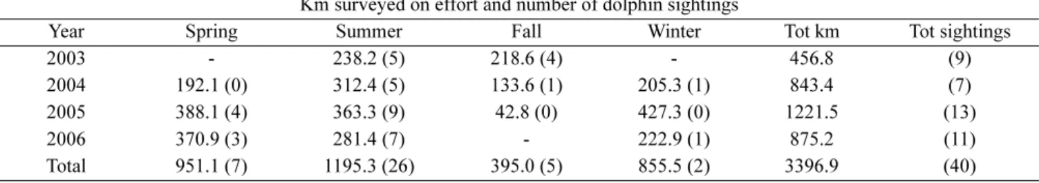
The stepwise logistic regression identified the most important predictors of dolphin presence in spring, summer and fall (Table 2). Low number of dolphin sightings in winter did not allow meaningful analyses in this season. Seven environmental covariates were selected by the model as significant predictors of dolphin presence: 1) mean oxygen saturation, 2) mean water temperature, 3) mean density anomaly, 4) gradient of density anomaly, 5) mean turbidity, 6) distance from the nearest coast and 7) bottom depth (Table 3).
Vessel speed, the only observer-dependent covariate selected by the model, was inversely correlated with dolphin presence in spring and directly in summer (Table 2). This unexpected result was thought to be the effect of an interaction between speed and slight differences in sea state recorded between these two seasons.
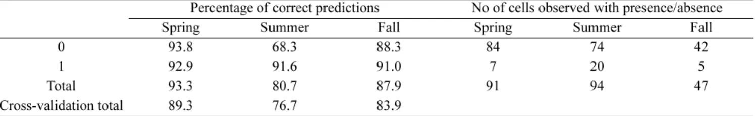
The model correctly predicted between 81% and 93% of the cells where animals were present, depending on season (Table 4). A leave-one-out cross-validation test was performed to check the accuracy of prediction. The results of the test indicated a good agreement between the model performances on both the training and cross-validation data sets. Agreement of training and cross-validation performances indicated a low risk of overfitting (Efron and Tibshirani 1993).
4. Discussion
The fact that bottlenose dolphins were the only cetacean species encountered during the surveys was expected and
consistent with previous studies conducted in this part of the Mediterranean Sea (Bearzi et al. 2004).
Variability caused by seasonal forcing is often a challenge in studies attempting to define habitat use by dolphins. Although many of the studies conducted so far have not taken this variable into account, seasonal differences are potentially important. For instance, in a recent study conducted in the northern California Current System, responses of several Odontocete species to biophysical
features and upwelling processes were both seasonally and spatially specific (Tynan et al. 2005). In one other study conducted off New Zealand, habitat selection by Hector’s dolphins was found to be affected by seasonal changes in sea surface temperature, water depth and water clarity (Bräger et al. 2003).
While species- and area-specific habitat preferences of cetaceans in terms of bathymetry and slope are apparent at the appropriate geographic scale of analysis (Notarbartolo di Sciara et al. 1993; Cañadas et al. 2002; Azzellino et al. 2008), patterns of habitat selection within relatively homogeneous dolphin habitats are poorly understood. The continental shelf waters of the study area – a typical habitat for bottlenose dolphins in the region (Notarbartolo di Sciara et al. 1993) – is relatively uniform in terms of bathymetry and sea floor features. However, this portion of the Adriatic Sea is characterized by high annual and seasonal variability of hydrological and biological variables (Franco and Michelato 1992; Socal et al. 2002; Grilli et al. 2005). This variability is thought to combine with the impact of local fisheries and determine wide shifts in the density and Table 2. Environmental predictors of dolphin presence based on a stepwise logistic regression. See text for description of abbreviated
variables.
Predictors of dolphin presence
SPRING B SE Wald P Exp(B) 95% CI
DistCoast −.059 .018 10.793 .001 .943 .910 .976 Speed −3.736 .212 311.173 .000 .024 .016 .036 DensityAn .732 .182 16.188 .000 2.080 1.456 2.971 Oxygen −.730 .062 137.627 .000 .482 .427 .544 Tmean −3.809 .270 199.068 .000 .022 .013 .038 Turbidity .239 .064 13.886 .000 1.270 1.120 1.440 DensityGr .101 .011 84.110 .000 1.106 1.083 1.130 Constant 161.254 12.780 159.201 .000
SUMMER B SE Wald P Exp(B) 95% CI
DistCoast −.021 .006 12.279 .000 .979 .968 .991 Speed .525 .059 80.065 .000 1.690 1.506 1.896 DensityAn −.276 .098 7.976 .005 .759 .627 .919 Oxygen .162 .009 362.427 .000 1.176 1.157 1.196 Turbidity −.071 .015 23.150 .000 .931 .905 .959 DensityGr −.029 .003 114.027 .000 .972 .967 .977 Depth −.104 .010 101.260 .000 .902 .884 .920 Constant −17.435 2.631 43.926 .000
FALL B SE Wald P Exp(B) 95% CI
Tmean 2.882 .532 29.346 .000 17.854 6.293 50.654
DensityGr −.040 .018 5.207 .022 .961 .928 .994
Depth .153 .039 14.946 .000 1.165 1.078 1.259
Constant −33.914 7.083 22.927 .000
Table 3. Environmental predictors of dolphin presence in different seasons. Signs ‘+’ and ‘−’ indicate direct and indirect correlation, respectively.
Predictors of dolphin presence: correlation
Spring Summer Fall
Oxygen − + Turbidity + − DistCoast − − DensityAn + − DensityGr + − − Depth − + Tmean − +
distribution of fish stocks (Bombace 1992). The northern Adriatic ecosystem is also especially sensitive to seasonal and long-term variations of anthropogenic nutrient loads (Degobbis et al. 2000) and climate (Russo et al. 2002). This study offered an opportunity to investigate the effects of hydrological variability on dolphin habitat use within an area of relatively uniform physiography. The stepwise procedure of the logistic regression analysis selected consistent predictors of dolphin presence in spring and summer (Table 3 and 4). However, the relationship (inverse or direct) between each predictor and dolphin presence varied between seasons, and different predictors were selected in fall. This indicates that dolphin distribution in the study area changed depending on seasonal forcing.
In spring, the plumes of main rivers become appreciable and their influence can be inferred from patterns of density, turbidity and dissolved oxygen. The spring temperature pattern is characterized by high spatial variability, with warm coastal waters influenced by riverine inputs and segregated water masses at the centre of the basin characterized by higher salinity and lower turbidity. Dolphins were predicted to occur closer to the coast but also in the open basin, as indicated by the selection of density anomaly as an important predictor. Moreover, the model showed an inverse correlation with temperature and a direct correlation with the density anomaly gradient, suggesting dolphin preference for the outer boundary of the front between river plumes and open waters. In summer, the dynamic of the basin is dominated by the Po river plume, with increased primary production caused by its nutrient loads (Degobbis et al. 2000). Density features reflect the mixing of oxygenated freshwater with saltier and denser waters of the open basin. Dolphin presence in summer was directly correlated with peaks of oxygen saturation and inversely correlated with water density. In fall, mean water temperature was the most relevant predictor. The highest
temperatures were found in the centre of the basin and consequently dolphin presence was also predicted at greater depths.
Although dolphin distribution and abundance are unlikely to be influenced directly by any of the variables considered in this study, dolphins may tend to concentrate in areas where hydrological features indirectly affect the density of their prey (Davis et al. 2002). The relationship between dolphin presence and high oxygen concentration in summer months, for instance, is a potentially important finding worth being validated by future studies. As saturation of dissolved oxygen may be regarded as a proxy for photosynthetic activity (Taylor et al. 1992), this result suggests that locally enhanced primary production may affect the availability of cetacean prey.
Prediction rates were relatively high in the three seasons considered, and particularly in spring (Table 4). However, these results should be taken with caution due to the relatively small sample size and short duration of the study, which prevented inclusion of winter in the analyses and further stratifications of the dataset (e.g. analyses of seasonal variations in different years). While this study should not be regarded as conclusive, information presented here flags a warning sign with regard to the simplistic inclusion of hydrological variables in studies of cetacean distribution and habitat selection in continental shelf areas. Modelling habitat use by coastal Odontocetes in areas characterized by extreme fluctuations due to input from rivers, complex hydrology, and high seasonal forcing, should rely on appropriate sets of hydrological and other variables and take into account seasonal variations. While scientists invariably look for simple patterns, in cases such as the one presented here complexity appears to be hard to set aside, and investigations of subtle patterns underlying habitat preference by dolphins (and possibly other top marine predators) should take into account the whole range of temporal variability.
Table 4. Percentage of cells where dolphin presence (1) and absence (0) were correctly predicted by the model in different seasons. ‘Cross-validation total’ refers to leave-one-out cross-validation test.
Percentage of correct predictions No of cells observed with presence/absence
Spring Summer Fall Spring Summer Fall
0 93.8 68.3 88.3 84 74 42
1 92.9 91.6 91.0 7 20 5
Total 93.3 80.7 87.9 91 94 47
5. Conclusion
This study shows that habitat modelling represents a promising but challenging way of predicting bottlenose dolphin presence based on hydrological and physiographical information in the northern Adriatic Sea. While the study area is relatively uniform in terms of bottom topography, dramatic seasonal variability in hydrological parameters results in changes of relevant predictors of dolphin presence from one season to another, and suggests highly variable patterns of distribution. Habitat use by the animals is influenced by complex interactions between hydrological variables, likely to determine seasonal and other shifts in prey distribution.
Acknowledgements
This work was funded in part through an INTERREG III CBC Phare Italy-Slovenia Project OBAS (Biological Oceanography of the northern Adriatic Sea). We are grateful to Leire Armentia Lasuen, Simona Bernasconi, Silvia Bonizzoni, Sebastiano Bruno, Annalise Petroselli and Nino Pierantonio for their contribution to the collection of field data. Vittorio Barale, Caterina Maria Fortuna, Giuseppe Notarbartolo di Sciara, Giorgio Socal and two anonymous reviewers offered useful suggestions to improve early drafts. Stefano Agazzi helped with the analyses and the maps.
References
Afifi, A. and V. Clark. 1996. Computer-aided multivariate analysis. Chapman & Hall, London.
Azzellino, A., S. Gaspari, S. Airoldi, and B. Nani. 2008. Habitat use and preferences of cetaceans along the continental slope and the adjacent pelagic waters in the western Ligurian Sea. Deep-Sea Res. I, 55, 296-323.
Baumgartner, M.F. 1997. The distribution of Risso’s dolphin (Grampus griseus) with respect to the physiography of the northern Gulf of Mexico. Mar. Mammal Sci., 13, 614-638. Bearzi, G., S. Agazzi, S. Bonizzoni, M. Costa, and A. Azzellino.
2008a. Dolphins in a bottle: Abundance, residency patterns and conservation of common bottlenose dolphins Tursiops truncatus in the semi-closed eutrophic Amvrakikos Gulf, Greece. Aquat. Conserv., 18(2), 130-146.
Bearzi, G., C.M. Fortuna, and R.R. Reeves. 2008b. Ecology and conservation of common bottlenose dolphins Tursiops truncatus in the Mediterranean Sea. Mamm. Rev. doi: 10.1111/j.1365-2907.2008.00133.x
Bearzi, G., D. Holcer, and G. Notarbartolo di Sciara. 2004. The role of historical dolphin takes and habitat degradation in shaping the present status of northern Adriatic cetaceans. Aquat. Conserv., 14, 363-379.
Bearzi, G., G. Notarbartolo di Sciara, and E. Politi. 1997. Social ecology of bottlenose dolphins in the Kvarneric (northern Adriatic Sea). Mar. Mammal Sci., 13, 650-668.
Bearzi, G., E. Politi, C.M. Fortuna, L. Mel, and G. Notarbartolo di Sciara. 2000. An overview of cetacean sighting data from the northern Adriatic Sea: 1987-1999. Eur. Res. Cetaceans, 14, 356-361.
Bearzi, G., E. Politi, and G. Notarbartolo di Sciara. 1999. Diurnal behavior of free-ranging bottlenose dolphins in the Kvarneric (northern Adriatic Sea). Mar. Mammal Sci., 15, 1065-1097. Bombace, G. 1992. Fisheries of the Adriatic Sea. p. 57-67. In:
Marine eutrophication and population dynamics, ed by G. Colombo, I. Ferrari, V.U. Ceccherelli, and R. Rossi. Olsen & Olsen, Fredensborg, Denmark.
Bräger, S., J.A. Harraway, and B.F.J. Manly. 2003. Habitat selection in a coastal dolphin species (Cephalorhynchus hectori). Mar. Biol., 143, 233-244.
Cañadas, A., R. Sagarminaga, R. De Stephanis, E. Urquiola, and P.S. Hammond. 2005. Habitat preference modelling as a conservation tool: proposals for marine protected areas for cetaceans in southern Spanish waters. Aquat. Conserv., 15, 495-521.
Cañadas, A., R. Sagarminaga, and S. García-Tiscar. 2002. Cetacean distribution related with depth and slope in the Mediterranean waters off southern Spain. Deep-Sea Res. I, 49, 2053-2073. Davis, R.W., J.G. Ortega-Ortiz, C.A. Ribi, W.E. Evans, D.C.
Biggs, P.H. Ressler, R.B. Cady, R.R. Leben, K.D. Mullin, and B. Würsig. 2002. Cetacean habitat in the northern oceanic Gulf of Mexico. Deep-Sea Res. I, 49, 121-142.
Degobbis, D., R. Precali, I. Ivancic, N. Smodlaka, D. Fuks and S. Kveder. 2000. Long-term changes in the northern Adriatic ecosystem related to anthropogenic eutrophication. Int. J. Environ. Pollut., 13, 495-533.
Efron, B. and R.J. Tibshirani. 1993. An introduction to the bootstrap. Chapman & Hall, London.
Evans, W.E. 1975. Distribution, differentiation of populations and other aspects of the natural history of Delphinus delphis Linnaeus in the Northeastern Pacific. Ph.D. Thesis, University of California, Los Angeles, CA. 145 p.
Ferguson, M.C., J. Barlow, P. Fiedler, S.B. Reilly, and T. Gerrodette. 2006. Spatial models of delphinid (family Delphinidae) encounter rate and group size in the eastern tropical Pacific Ocean. Ecol. Model., 193, 645-662.
Fiedler, P.C., J. Barlow, and t. Gerrodette. 1998. Dolphin prey abundance determined from acoustic backscatter data in eastern pacific surveys. Fishery Bull., 96, 237-247.
dolphins (Tursiops truncatus) in the north-eastern Adriatic Sea. Ph.D. Thesis, University of St. Andrews, U.K. 250 p. Franco, P. and A. Michelato. 1992. Northern Adriatic Sea:
oceanography of the basin proper and of the western coastal zone. Sci. Total Environ. Suppl., 35-62.
Goold, J.C. 1998. Acoustic assessment of populations of common dolphin off the west Wales coast, with perspectives from satellite infrared imagery. J. Mar. Biol. Assoc. U.K., 78, 1353-1364.
Griffin, R.B. and N.J. Griffin. 2003. Distribution, habitat partitioning, and abundance of Atlantic spotted dolphins, bottlenose dolphins, and loggerhead sea turtles on the eastern Gulf of Mexico continental shelf. Gulf of Mexico Science, 2003, 23-34. Grilli, F., M. Marini, D. Degobbis, C.R. Ferrari, P. Fornasiero, A.
Russo, M. Gismondi, T. Djakovac, R. Precali, and R. Simonetti. 2005. Circulation and horizontal fluxes in the northern Adriatic Sea in the period June 1999-July 2002. Part II: Nutrients transport. Sci. Total Environ., 353, 115-125.
Guisan, A. and N.E. Zimmermann. 2000. Predictive habitat distribution models in ecology. Ecol. Model., 135, 147-186. Hooker, S.K., H. Whitehead, and S. Gowans. 1999. Marine
Protected Area design and the spatial and temporal distribution of cetaceans in a submarine canyon. Cons. Biol., 13, 592-602. Hosmer, D.W. and S. Lemeshow. 2000. Applied logistic regression,
2nd Ed. John Wiley & Sons, New York.
Hui, C.A. 1979. Undersea topography and distribution of dolphins of the genus Delphinus in the Southern California bight. J. Mammal., 60, 521-527.
Hui, C.A. 1985. Undersea topography and the comparative distributions of two pelagic cetaceans. Fishery Bull., 83, 472-475.
Kruskal, W.H. and W.A. Wallis. Use of ranks in one-criterion variance analysis. J. Am. Stat. Assoc., 47, 583-621.
Mullin, K.D., W. Hoggard, C.L. Roden, R.R. Lohoefener, C.M. Rogers, and B. Taggart. 1994. Cetaceans on the upper continental slope in the north-central Gulf of Mexico. Fishery Bull., 92, 773-786.
Notarbartolo Di Sciara, G., M.C. Venturino, M. Zanardelli, G. Bearzi, J.F. Borsani, and B. Cavalloni. 1993. Cetaceans in the central Mediterranean Sea: distribution and sighting frequencies. Ital. J. Zool., 60, 131-138.
Polacheck, T. 1987. Relative abundance, distribution and inter-specific relationship of cetacean schools in the Eastern Tropical Pacific. Mar. Mammal Sci., 13, 614-638.
Pugnetti, A., F. Acri, L. Alberighi, D. Barletta, M. Bastianini, F.
Bernardi-Aubry, A. Berton, F. Bianchi, G. Socal, and C. Totti. 2004. Phytoplankton photosynthetic activity and growth rates in the NW Adriatic Sea. Chem. Ecol., 2, 399-409. Reilly, S.B. 1990. Seasonal changes in distribution and habitat
differences among dolphins in the eastern tropical Pacific. Mar. Ecol. Prog. Ser., 66, 1-11.
Russo, A., S. Rabitti, and M. Bastianini. 2002. Decadal climatic anomalies in the northern Adriatic Sea inferred from a new oceanographic data set. Mar. Ecol. Evol. Persp., 23, 340-351.
Selzer, L.A. and P.M. Payne. 1988. The distribution of white-sided (Lagenorhynchus acutus) and common dolphins (Delphinus delphis) vs. environmental features of the continental shelf of the northeastern United States. Mar. Mammal Sci., 4, 141-153.
Shane, S.H. 1990. Comparison of bottlenose dolphin behavior in Texas and Florida, with a critique of methods for studying dolphin behavior. p. 541-558. In: The bottlenose dolphin, ed. by S. Leatherwood and R.R. Reeves. Academic Press, San Diego, CA.
Silber, G.K., M.W. Newcomer, P.C. Silber, H. Pérez-Cortés, and G.M. Ellis. 1994. Cetaceans of the northern Gulf of California: distribution, occurrence, and relative abundance. Mar. Mammal Sci., 10, 283-298.
Socal, G., A. Pugnetti, and L. Alberighi. 2002. Observations on phytoplankton productivity in relation to hydrography in NW Adriatic. Chem. Ecol., 18, 61-73.
Taylor, A.H., A.J. Watson, and J.E. Robertson. 1992. The influence of the spring phytoplankton bloom on carbon dioxide and oxygen concentrations in the surface waters of the northeast Atlantic during 1989. Deep-Sea Res. I, 39, 137-152. Tynan, C.T., D.G. Ainley, J.A. Barth, T.J. Cowles, S.D. Pierce,
and L.B. Spear. 2005. Cetacean distributions relative to ocean processes in the northern California Current System. Deep-Sea Res. II, 52, 145-167.
Webster, R. and M.A. Oliver. 2001. Geostatistics for environmental scientists. Statistics in Practice series. John Wiley & Sons, Chichester, U.K.
Yen, P.W., W.J. Sydeman, and K.D. Hyrenbach. 2004. Marine bird and cetacean associations with bathymetric habitats and shallow-water topographies: implications for trophic transfer and conservation. J. Marine Syst., 50, 79-99.
Zavatarelli, M., F. Raicich, D. Bregant, A. Russo, and A. Artegiani. 1998. Climatological biogeochemical characteristics of the Adriatic Sea. J. Marine Syst., 18, 227-263.