ABSTRACT Quantitative data of 50 non-polar organic compounds constituting PM2.5
were continuously collected and analyzed from June 2016 to October 2017
(approxi-mately 17 months) at Ichihara, one of the largest industrial areas in Japan. Target non-polar organic compounds including 21 species of polycyclic aromatic hydrocarbons
(PAHs), 24 species of n-alkanes and 5 species of phthalate esters(PAEs) were
simultane-ously measured by gas chromatography/mass spectrometry. Basically, the average con-centrations of the total PAHs, n-alkanes and PAEs in each season remained nearly level, and seasonal variations were little throughout the study period. These results suggest that the emission sources, which are not influenced by the seasons, are the dominant inputs for the target organic compounds. Diagnostic ratios of PAHs, assessment of n-alkane homologue distributions, carbon preference index, and the contribution of wax n-alkanes from plants were used to estimate source apportionments. These results indi-cate that anthropogenic sources were the main contributor for most PAHs and n-alkanes throughout the study period. The concentrations of PAEs selected in this study were low because emission amounts of these chemicals were little within the source areas of the sampling site. To our knowledge, this study is the first attempt to simultaneously
mea-sure a high number of non-polar organic compounds in PM2.5 collected from the
ambi-ent air of Japan, and the resultant data will provide valuable data and information for environmental researchers.
KEY WORDS PM2.5, Polycyclic aromatic hydrocarbons, n-Alkanes, Phthalate esters, Organic compounds, Japan
1. INTRODUCTION
Particulate matter(PM) is an atmospheric pollutant that has received wide-spread concern as it causes public health problems and plays important roles in regulating regional and global climate(Fuzzi, et al., 2015; IPCC, 2013; WHO,
2013; Jacob, 1999). Among the PM, particle sizes with aerodynamic diameter less than 2.5μm(PM2.5) are particularly hazardous to public health because of their
Measurements of 50 Non-polar Organic Compounds Including
Polycyclic Aromatic Hydrocarbons, n-Alkanes and Phthalate Esters in
Fine Particulate Matter (PM
2.5) in an Industrial Area of Chiba
Prefecture, Japan
Yujiro Ichikawa*, Takehisa Watanabe, Yasuhide Horimoto, Katsumi Ishii, Suekazu Naito
Chiba Prefectural Environmental Research Center, 1-8-8 Iwasaki Nishi, Ichihara, Chiba 290-0046, Japan
*Corresponding author. Tel: +81-436-21-6371 E-mail: [email protected]
Current affiliation
Chiba Prefectural Environmental and Community Affairs Department Air Quality Division, 1-1 Ichiba-cho, Chuo-ku, Chiba, Chiba 260-8667, Japan Tel: +81-43-223-3804
Received: 29 March 2018
Revised: 1 June 2018
Accepted: 27 June 2018
www.asianjae.org
Vol. 12, No. 3, pp. 274-288, September 2018 doi: https://doi.org/10.5572/ajae.2018.12.3.274
ISSN(Online) 2287-1160, ISSN(Print) 1976-6912
Technical Information
Copyright © 2018 by Asian Journal of Atmospheric Environment
This is an open-access article distributed under the terms of the Creative Commons Attribution Non-Commercial License(http://creativecommons.
org/licenses/by-nc/4.0/), which permits unrestricted non-commercial use, distribution, and reproduction in any medium, provided the original work is properly cited.
ability to penetrate into the alveoli of lungs and they are therefore more likely to increase the incidence of respira-tory and cardiovascular diseases(Ueda, 2011; Schwartz and Neas, 2000).
According to the information provided by the Minis-try of the Environment Japan, 74.5% of stations toring general ambient air, and 58.4% of stations moni-toring auto-exhaust emissions met environmental quali-ty standards for PM2.5 during the 2015 fiscal year(from
April to March of the following year), and further coun-termeasures to reduce the level of PM2.5 are required
(http://www.env.go.jp/press/103858.html, in Japanese, Accessed on June 1, 2018). For an effective reduction of PM2.5 levels, it is important to identify their emission
sources and describe their chemical properties in the ambient air. Long time series of quantitative data of the chemical compositions that constitute PM2.5 are
neces-sary to provide the required information to achieve PM2.5 reduction.
Along with chemical compounds that are utilized for the assessment of PM2.5 emission sources(e.g., trace
metals), some organic compounds have definitive chem-ical structures that can be correlated to emission sources and are known as molecular markers. They can originate from many sources, including combustion of fossil fuels, biogenic origin, biomass burning, motor vehicles, waste incineration, steel/plastic manufacturing, cooking, and road dust(Hayakawa et al., 2016; Kawamura and
Bikki-na, 2016; Wang et al., 2016; Zhang et al., 2013; Alves et al., 2009; Alves, 2008; Brandenberger et al., 2005; He et al., 2004; Simoneit, 2002; Oros et al., 1999; Khalili et al.,
1995; Rogge et al., 1993a, 1993b, 1993c; Simoneit et al.,
1991).
A wealth of publications have reported that the organ-ic fraction of PM2.5 consists of various kinds of organic
compounds with different abundances in different areas of the world(Ichikawa et al., 2017; Mikuška et al.,
2017; Ahmed et al., 2016; Fang et al., 2016; Li et al.,
2016; Alves et al., 2015; Yadav et al., 2013; Park et al.,
2006; Simoneit et al., 2004). Moreover, increasing
atten-tion has been paid to the study of the organic com-pounds in PM2.5 to improve under standing of the
emis-sion sources and source apportionment. However, in Japan, most PM2.5 studies have focused on metallic
ele-ments, carbonaceous components, and water-soluble inorganic components, and studies into organic com-pounds remain deficient.
Therefore, we intensively measured 50 different non-polar organic compounds including 21 species of poly-cyclic aromatic hydrocarbons(PAHs), 24 species of n-alkanes and 5 species of phthalate esters(PAEs) in PM2.5 in a long time series at Ichihara, a major industrial
area in Japan. Selected non-polar organic compounds were simultaneously measured employing GC/MS. To the best of our knowledge, this paper is the first attempt to simultaneously measure as many non-polar organic compounds in PM2.5 collected for a long time series
(approximately 17 months) from the ambient atmo-sphere of Japan. Our results aim to provide useful insights and data for use in improving understanding of the target organic compounds in PM2.5 and thereby
contribute to better air quality management strategies.
2. MATERIALS AND METHODS
2.1 Sampling Site Description
Sampling was conducted on the roof(12m height above the ground) of the Chiba Prefectural Environ-mental Research Center(CERC). The CERC is locat-ed between the industrial zone of Tokyo Bay(a large industrial base including gas power plants, heavy petro-chemical industries, and many light industries within ca. 2km radius), and the residential zone of Ichihara, Chiba Prefecture, Japan(Fig. 1). The site is located approximately 200 m southeast of the Japanese Nation-al Route 16(average weekday 24-hour traffic of 42,007 vehicles, of which 29.1% are large-sized vehicles). Ichi-hara is about 40 km southeast of central Tokyo, and the estimated population is nearly 277,000.
2.2 Sample Collection
PM2.5 samples were collected on 47mm diameter
quartz filter(Pall Corp., 2500QAT-UP, Q-filter) from 13 June 2016 to 25 October 2017. The flow rate of the low volume air sampler(Rupprecht and Patashnick Co., Inc., Partisol-FRM Model 2000 Air Sampler) was
16.7 L/min with a constant sampling rate (accumulat-ing to ca. 24m3/d). From our previous study, daily air
volumes per sample(24 m3/d) were too low to
quanti-fy some of the organic compounds present in relatively small amounts in the ambient atmosphere, so the sam-ples in this study were sampled on a weekly basis (Ichikawa et al., 2017). Park et al.(2006) also pointed out the difficulty of detailed analysis of organic com-pounds by gas chromatography/mass spectrometry (GC/MS) from daily sampling, supporting the decision to analyze samples on a weekly basis. Some amount of organic compounds may be decomposed or evaporated from the Q-filter during the sampling. However, due to the reason mentioned above those were not taken into consideration in this study.
The sampling periods are described in Table 1. Based on the definition used by the Japanese Meteorological Agency, the four seasons were assigned as follows: March to May for spring, June to August for summer, September to November for autumn and December to February for winter.
Typically, Q-filters are combusted in a furnace with high temperatures to remove the existing organic car-Table 1. Details of sampling period in each season.
Year Season*1) Sampling period n
2016
Summer Jun. 13-Jul. 20Jul. 4-Jul. 11 Jun. 20-Jun. 27Jul. 11-Jul. 18 Jun. 28-Jul. 4Aug. 22-Aug. 29 6
Autumn Aug. 29-Sep. 5 Sep. 20-Sep. 27 Oct. 17-Oct. 25 Nov. 8-Nov. 15 Sep. 5-Sep. 12 Oct. 3-Oct. 11 Oct. 25-Nov. 1 Nov. 15-Nov. 22 Sep. 12-Sep. 20 Oct. 11-Oct. 17 Nov. 1-Nov. 8 Nov. 29-Dec. 2 12 Winter Dec. 2-Dec. 7 Dec. 21-Dec. 28 Jan. 11-Jan. 18 Jan. 31-Feb. 8 Feb. 22-Mar. 1 Dec. 7-Dec. 14 Dec. 28-Jan. 4 Jan. 18-Jan. 25 Feb. 8-Feb. 15 Dec. 14-Dec. 21 Jan. 5-Jan. 10 Jan. 25-Jan. 31 Feb. 15-Feb. 22 13 2017 Spring Mar. 1-Mar. 8 Mar. 22-Mar. 29 Apr. 12-Apr. 19 May 2-May 10 May 24-May 31 Mar. 8-Mar. 15 Mar. 29-Apr. 5 Apr. 19-Apr. 26 May 10-May 17 Mar. 15-Mar. 22 Apr. 5-Apr. 12 Apr. 26-May 2 May 17-May 24 13 Summer May 31-Jun. 7 Jun. 21-Jun. 28 Jul. 12-Jul. 19 Aug. 2-Aug. 8 Aug. 23-Aug. 30 Jun. 7-Jun. 14 Jun. 28-Jul. 5 Jul. 19-Jul. 26 Aug. 8-Aug. 16 Jun. 14-Jun. 21 Jul. 5-Jul. 12 Jul. 26-Aug. 2 Aug. 16-Aug. 23 13
Autumn Aug. 30-Sep. 4Sep. 20-Sep. 27 Oct. 11-Oct. 17 Sep. 4-Sep. 12 Sep. 27-Oct. 4 Oct. 17-Oct. 25 Sep. 12-Sep. 20 Oct. 4-Oct. 11 8
bon(OC) prior to sampling. However, combustion could activate the Q-filter, resulting in positive artifacts due to the absorption of gas phase organic materials onto the filter. As described in Section 2.3, gravimetric measurements of PM2.5 collected in Q-filters were
designed in this study and to eliminate the possible positive artifacts during transport, sampling and stor-age, Q-filters were not combusted.
Travel blank filters were prepared and placed in the same container as the samples and were transported and treated in the same way(e.g., making contact with the sampling devices, and being exposed to the conditions of the sampling site, storage, and all analytical procedures). Sample results reported in this paper were corrected based on the travel blank filters.
Sample filters were placed in petri dishes and enclosed in a sealed bag. All samples were stored in a freezer at -30°C until chemical analysis to prevent evaporation and degradation of components constituting PM2.5. A
total of 68 effective samples were collected in this study, which included 3 blank samples.
2.3 PM2.5 Mass Concentration
Both PM2.5 sample filters and travel blank filters were
weighed using an electronic microbalance(A&D Com-pany Ltd., BM-20) with a reading precision of 1μg. Prior to weighing, all Q-filters were kept under equili-brated conditions of constant temperature(21.5± 1.5°C) and relative humidity(35±5%) for at least 24 hours. An ionizing blower was used to eliminate the effects of static electricity on the weighing process. Obtained PM2.5 mass(μg) was calculated by
subtract-ing pre-weight from post-weight of the Q-filters. The PM2.5 mass concentrations(μg/m3) were calculated by
PM2.5 mass per total volume of suction.
For the accuracy testing of gravimetric measurement, PM2.5 mass concentration was measured in parallel using
an automatic instrument(Horiba Ltd., APDA-3750A) employing a beta-ray absorption technique. Automatic instrument was installed at the monitoring station of the CERC, at a height of 7m above the ground. PM2.5 mass
concentrations observed by two different methodologies showed good positive correlation(n=64, R=0.84).
2.4 OC Measurement
The OC was measured by the thermal/optical reflec-tance carbon analysis system(Sunset Laboratory Inc., Lab OC-EC Aerosol Analyzer). The analytical
condi-tions of the IMPROVE method(Chow et al., 1993) were
used with the thermal optical reflection protocol(Chow
et al., 2001). A total of four fractions(OC1, OC2, OC3, and OC4) and the optical pyrolysis correction of OC (PyC) were determined. The OC was calculated as OC1+OC2+OC3+OC4+PyC.
2.5 Organic Compounds Measurement
The measured non-polar organic compounds in this study were 21 species of PAHs, 24 species of n-alkanes and 5 species of PAEs, producing a total of 50 species. Details of these compounds, including individual abbre-viations, are presented in Tables 2 and 3.
2.5.1 Pretreatment Procedure
A Q-filter was placed in a 10mL glass flask with stop-per and spiked with defined amounts of the internal standard(IS) substances. The IS substances employed in this study were as follows. For PAHs: anthracene-d10
(Ant-d10), pyrene-d10(Py-d10), benzo(a)pyrene-d12
(BaP-d12), and benzo(g,h,i)perylene-d12(BghiP-d12).
For n-alkanes: n-tetracosane-d50(C24-d50). For PAEs:
diethyl phthalate-d4 (DEP-d4), di-n-butyl phthalate-d4
(DBP-d4), bis(2-ethylhexyl)adipate-d8(DEHA-d8), and
benzyl butyl phthalate-d4(BBP-d4). Samples were
extracted in 5mL dichloromethane solution twice using an ultrasonic bath for 15min, followed by filtration through a hydrophilic PTFE syringe filter(ADVANTEC Co. Ltd., DISMIC, pore size of 0.22μm) to remove inso-luble particles and quartz fibers. The extracts were evap-orated to dryness under a gentle stream of high purity nitrogen gas and re-dissolved in 100μL of toluene for GC/MS analysis.
2.5.2 GC/MS Analysis
Analysis of the target organic compounds in the PM2.5
samples was carried out by GC/MS(6890 GC/5973 MSD, Agilent Technology) under the following condi-tions: capillary column DB-5MS(length; 60m, internal dia meter; 0.25mm, film thickness; 0.25μm film thick-ness, Agilent J&W) was used for separation of the com-pounds; high-purity helium was used as the carrier gas with flow rate of 1.0mL/min; sample injection amount was 1μL in splitless mode; the GC oven temperature was initially held at 100°C for 1min, increasing 20°C/ min until 270°C and held for 17min, increasing 15°C/ min until 320°C and then held for 32min; the injection temperature was set to 280°C and the MS source and
Table 2. T empe ra tur e, l imit of de te ct ion of P A H s (n g/m 3), r ec ov er y p er ce nt ag es o f P A H s (% ), c onc en tr at ion s of P M2.5 (μg/m 3), O C (μg/m 3), a nd P A H s (n g/m 3); r at io s o f P A H s ac coun tin g for P M2.5 and O C; a nd d ia gnos tic r at ios be tw ee n P AH s. C ompound s a nd ra tios Ab br e v ia tion U nit R eco ve ry (% ) (n = 4) LO D R an ge Av er ag e Summe r 2016 (n= 6) Autumn 2016 (n= 12) W int er 2016 (n=13) Spr in g 2017 (n=13) Summe r 2017 =(n13) Autumn 2017 =(n 8) Tot al (n = 65) Summe r 2016 Autumn 2016 W int er 2016 Spr in g 2017 Summe r 2017 Autumn 2017 Tot al Te mpe ra tur e °C 17.5-36.6 − 0.4-32.4 − 3.5-21.3 − 0.8-29.4 14.7-36.4 10.5-32.2 − 3.5-36.6 25.4 18.8 7.9 14.4 25.3 20.7 18.5 PM 2.5 μg/m 3 4.4-11 5.3-15 7.0-16 9.4-16 6.2-14 4.9-9.4 4.4-16 7.5 10 11 12 9.0 7.4 9.9 OC μg/m 3 0.81-1.3 0.80-3.3 1.3-3.7 1.1-2.4 0.66-3.1 1.0-1.9 0.66-3.7 0.96 1.9 2.3 1.8 1.3 1.4 1.7 O C/P M2.5 % 9.4-18 12-28 17-26 11-19 11-22 14-22 9.4-28 13 19 20 15 14 19 17 PA H s Fluor ene Fl ng/m 3 88 0.013 N .D. *1)-N .D. N .D .-N .D . N .D .-0.070 0.020-0.067 N .D .-0.066 N .D .-0.033 N .D .-0.070 N .D. N .D. 0.035 0.033 0.020 0.023 0.022 Ph en ant hr en e Ph e ng/m 3 96 0.0096 N .D .-0.024 N .D .-0.021 0.045-0.30 0.016-0.24 N .D .-0.066 N .D .-0.043 N .D .-0.30 0.0080 0.0069 0.16 0.11 0.021 0.022 0.063 An thr ac ene Ant ng/m 3 97 0.016 N .D .-0.034 N .D .-N .D . N .D .-0.22 N .D .-0.016 N .D .-0.094 N .D .-N .D . N .D .-0.22 0.012 N .D. 0.044 0.0084 0.021 N .D. 0.018 Fluor an the ne Fluor ng/m 3 97 0.0077 0.14-0.56 0.092-0.53 0.22-0.96 0.16-0.69 0.094-0.57 0.11-0.24 0.092-0.96 0.30 0.22 0.50 0.45 0.23 0.17 0.33 Py re ne Py ng/m 3 98 0.009 0.12-0.54 0.082-0.43 0.18-0.82 0.14-0.61 0.084-0.55 0.097-0.21 0.082-0.82 0.28 0.19 0.40 0.39 0.21 0.15 0.28 Be nz o( c)p he na nthr ene BcP ng/m 3 90 0.063 N .D .-N .D . N .D .-N .D . N .D .-N .D . N .D .-N .D . N .D .-N .D . N .D .-N .D . N .D .-N .D . N .D. N .D. N .D. N .D. N .D. N .D. N .D. Be nz( a)a nthr ac ene Ba A ng/m 3 99 0.032 0.067-0.18 0.052-0.16 0.038-0.14 0.037-0.12 N .D .-0.16 N .D .-0.043 N .D .-0.18 0.11 0.083 0.082 0.074 0.057 0.026 0.071 C hr ys ene Ch ry ng/m 3 88 0.057 N .D .-0.35 N .D .-0.13 N .D .-0.35 0.059-0.27 N .D .-0.34 N .D .-N .D . N .D .-0.35 0.14 0.066 0.17 0.16 0.098 N .D. 0.11 Be nz o( b)f luor an the ne Bb F ng/m 3 95 0.037 0.17-0.84 0.10-0.46 0.14-0.89 0.17-0.47 N .D .-0.75 0.11-0.20 N .D .-0.89 0.37 0.27 0.45 0.33 0.24 0.16 0.31 7,12-Dime th yl be nz (a )a nthr ac ene 7,12D aA ng/m 3 90 0.038 N .D .-N .D . N .D .-N .D . N .D .-N .D . N .D .-N .D . N .D .-N .D . N .D .-N .D . N .D .-N .D . N .D. N .D. N .D. N .D. N .D. N .D. N .D. Be nz o( j)f luor an the ne Bj F ng/m 3 89 0.051 0.082-0.33 0.065-0.19 0.087-0.38 0.089-0.23 0.054-0.40 0.065-0.15 0.054-0.40 0.16 0.12 0.22 0.16 0.14 0.10 0.15 Be nz o( k)f luor an the ne Bk F ng/m 3 90 0.040 0.088-0.35 0.072-0.23 0.08-0.31 0.080-0.21 N .D .-0.32 0.045-0.097 N .D .-0.35 0.17 0.13 0.18 0.15 0.10 0.069 0.13 Be nz o( e)p yr ene BeP ng/m 3 92 0.019 0.13-0.70 0.090-0.35 0.11-0.61 0.12-0.37 0.094-0.75 0.096-0.18 0.09-0.75 0.30 0.21 0.31 0.25 0.24 0.14 0.24 Be nz o( a)p yr ene Ba P ng/m 3 96 0.024 0.17-0.81 0.15-0.46 0.12-0.68 0.13-0.45 0.13-0.86 0.13-0.24 0.12-0.86 0.36 0.26 0.30 0.28 0.30 0.18 0.28 3-M eth ylcho la nthr ene 3MC ng/m 3 100 0.046 N .D .-N .D . N .D .-N .D . N .D .-N .D . N .D .-N .D . N .D .-N .D . N .D .-N .D . N .D .-N .D . N .D. N .D. N .D. N .D. N .D. N .D. N .D. Inde no(1,2,3-cd )p yr ene IP ng/m 3 100 0.026 0.13-0.94 N .D .-0.45 0.13-0.85 0.15-0.46 0.12-1.1 0.12-0.25 N .D .-1.1 0.37 0.29 0.41 0.30 0.33 0.20 0.32 Di be nz( a,h )a nthr ac ene DB ahA ng/m 3 100 0.019 0.054-0.19 0.043-0.14 N .D .-0.13 N .D .-0.072 N .D .-0.15 N .D .-0.040 N .D .-0.19 0.097 0.088 0.06 0.046 0.047 0.030 0.060 Be nz o(g ,h, i)pe ry le ne BghiP ng/m 3 96 0.013 0.11-0.82 0.078-0.39 0.14-0.80 0.14-0.41 0.11-0.88 0.12-0.24 0.078-0.88 0.32 0.27 0.40 0.29 0.29 0.19 0.30 Di be nz o( a,l )p yr ene DB alP ng/m 3 100 0.036 0.049-0.26 0.054-0.17 N .D .-0.21 N .D .-0.098 N .D .-0.24 N .D .-0.046 N .D .-0.26 0.11 0.11 0.098 0.063 0.060 0.032 0.079 Di be nz o( a, i)p yr ene DB aiP ng/m 3 110 0.056 N .D .-0.19 0.12-0.31 N .D .-N .D . N .D .-N .D . N .D .-0.070 N .D .-N .D . N .D .-0.31 0.13 0.15 N .D. N .D. 0.031 N .D. 0.061 Di be nz o( a,h )p yr ene DB ahP ng/m 3 100 0.059 N .D .-0.11 N .D .-0.11 N .D .-N .D . N .D .-N .D . N .D .-N .D . N .D .-N .D . N .D .-0.11 0.075 0.047 N .D. N .D. N .D. N .D. 0.037 ΣPA H s *2) ng/m 3 1.6-7.3 1.3-4.5 1.7-7.6 1.7-4.7 1.1-7.4 1.1-2.1 1.1-7.6 3.4 2.6 4.0 3.2 2.5 1.6 2.9 ΣP AH s/P M2.5 % 0.026-0.073 0.018-0.041 0.024-0.057 0.011-0.040 0.013-0.053 0.015-0.032 0.011-0.073 0.043 0.027 0.035 0.027 0.027 0.023 0.030 ΣP AH s/O C % 0.20-0.55 0.062-0.35 0.097-0.25 0.074-0.33 0.065-0.37 0.089-0.16 0.062-0.55 0.33 0.16 0.18 0.19 0.20 0.12 0.19 Σ3-rin gs *3) ng/m 3 0.019-0.065 0.019-0.035 0.093-0.43 0.052-0.29 0.019-0.18 0.019-0.074 0.019-0.43 0.027 0.021 0.24 0.15 0.062 0.053 0.10 Σ4-rin gs *4) ng/m 3 0.41-1.7 0.31-1.3 0.52-2.3 0.45-1.7 0.27-1.7 0.30-0.57 0.27-2.3 0.88 0.62 1.2 1.1 0.65 0.42 0.84 Σ5-rin gs *5) ng/m 3 0.72-3.2 0.54-1.9 0.57-3.0 0.62-1.8 0.44-3.3 0.48-0.91 0.44-3.3 1.5 1.1 1.5 1.3 1.1 0.70 1.2 Σ6-rin gs *6) ng/m 3 0.35-2.3 0.38-1.3 0.35-1.9 0.37-1.0 0.32-2.3 0.32-0.57 0.32-2.3 1.0 0.88 0.96 0.71 0.75 0.48 0.80 BeP/( BeP + Ba P) 0.42-0.46 0.38-0.54 0.47-0.58 0.44-0.53 0.41-0.47 0.40-0.46 0.38-0.58 0.44 0.46 0.51 0.48 0.44 0.44 0.46 Ba A/ (Ba A + C hr) 0.34-0.70 0.48-0.71 0.29-0.57 0.29-0.41 0.30-0.65 0.36-0.60 0.29-0.71 0.52 0.58 0.35 0.33 0.42 0.46 0.43 IP/( IP +BghiP ) 0.52-0.56 0.042-0.56 0.48-0.52 0.49-0.53 0.48-0.56 0.46-0.56 0.042-0.56 0.54 0.49 0.51 0.50 0.52 0.51 0.51 Fluor/( Flour +Py) 0.51-0.55 0.50-0.56 0.52-0.57 0.52-0.57 0.50-0.54 0.53-0.55 0.50-0.57 0.53 0.54 0.55 0.54 0.52 0.54 0.54 BghiP/B aP 0.65-1.0 0.52-1.6 1.2-1.7 0.91-1.5 0.76-1.3 0.92-1.2 0.52-1.7 0.81 1.1 1.3 1.1 0.99 1.1 1.1 Exc
ept for the t
empe ra tur e, al l of the me as ur ed v alue s h av e be en r ounde d t o no mor e th an thr ee si gni fica nt f ig ur es . *1) N .D . : N ot de te ct ed ( be lo w L OD ) *2) Σ PA H s= Fl + Ph e+ Ant + Fluor + Py + BcP + Ba A + Ch ry + Bb F + 7,12D aA + Bj F + Bk F + BeP + Ba P + 3MC + IP + DB ahA + BghiP + DB alP + DB aiP + DB ahP *3) Σ 3-rin gs =Fl +Ph e+ Ant *4) Σ 4-rin gs = Fluor + Py + BcP + Ba A + Ch ry + 7,12D aA *5) Σ 5-rin gs =Bb F +Bj F +Bk F +BeP +Ba P +3MC +DB ahA *6) Σ 6-rin gs = IP + BghiP + DB alP + DB aiP + DB ahP
Table 3. L OD of n-al ka ne s a nd P A Es (n g/m 3), r ec ov er y pe rc en ta ge s of n-al ka ne s a nd P A Es (% ), c onc en tr at ion s of n-al ka ne s a nd P A Es (n g/m 3) a nd ra tios of n-al ka ne s a nd P A Es ac coun tin g for P M2.5 and O C . C ompound s, ra tios a nd index Ab br ev ia tion U nit R eco ve ry (% ) (n = 4) LO D R an ge Av er ag e Summe r 2016 (n =6) Autumn 2016 (n =12) W in te r 2016 (n =13) Spr in g 2017 (n =13) Summe r 2017 (n =13) Autumn 2017 (n =8) Tot al (n =65) Summe r 2016 Autumn 2016 W int er 2016 Spr in g 2017 Summe r 2017 Autumn 2017 Tot al n-Al ka ne s n-H ept ade ca ne C17 ng/m 3 87 0.0095 0.025-0.076 0.014-0.15 0.052-0.19 0.028-0.15 N .D. *1)-0.050 N .D .-0.067 N .D .-0.19 0.044 0.050 0.11 0.065 0.027 0.017 0.056 n-O ct ade ca ne C18 ng/m 3 78 0.0072 0.016-0.071 0.014-0.060 0.027-0.12 0.018-0.094 N .D .-0.27 N .D .-0.058 N .D .-0.27 0.037 0.030 0.066 0.046 0.080 0.023 0.050 n-N on ade ca ne C19 ng/m 3 84 0.0042 0.016-0.060 0.014-0.096 0.054-0.16 0.018-0.095 0.0051-0.11 N .D .-0.050 N .D .-0.16 0.035 0.041 0.09 0.047 0.026 0.024 0.046 n-Eic os ane C20 ng/m 3 89 0.0062 0.021-0.085 0.014-0.15 0.067-0.23 0.0071-0.12 N .D .-0.14 0.0080-0.069 N .D .-0.23 0.048 0.061 0.13 0.052 0.027 0.029 0.061 n-H eneic os ane C21 ng/m 3 96 0.0055 0.014-0.13 0.021-0.30 0.10-0.47 0.0096-0.21 0.0089-0.29 0.013-0.063 0.0089-0.47 0.068 0.099 0.21 0.086 0.050 0.034 0.098 n-D oc os ane C22 ng/m 3 110 0.0076 0.016-0.24 0.029-0.72 0.22-0.78 N .D .-0.41 N .D .-0.70 0.0098-0.22 N .D .-0.78 0.12 0.20 0.46 0.17 0.088 0.063 0.20 n-Tr ic os ane C23 ng/m 3 120 0.0059 0.054-0.41 0.094-1.0 0.44-1.9 0.056-0.73 0.041-1.7 0.063-0.25 0.041-1.9 0.25 0.31 0.84 0.32 0.23 0.13 0.37 n-Te tra cos ane C24 ng/m 3 130 0.0071 0.085-0.66 0.011-1.7 0.75-2.5 0.042-1.5 N .D .-3.7 0.068-0.62 N .D .-3.7 0.37 0.50 1.5 0.55 0.46 0.33 0.66 n-Pent ac os an e C25 ng/m 3 120 0.010 0.35-1.0 0.13-2.1 1.1-3.2 0.46-1.8 0.21-6.2 0.30-1.2 0.13-6.2 0.68 1.0 2.0 1.0 0.96 0.64 1.1 n-H ex ac os ane C26 ng/m 3 110 0.0097 0.41-1.2 0.29-2.3 0.9-3.2 0.62-2.0 0.33-6.4 0.61-1.4 0.29-6.4 0.81 1.2 1.8 1.0 1.1 0.92 1.2 n-H ept ac os ane C27 ng/m 3 110 0.0061 0.40-2.1 0.37-2.8 0.63-3.7 0.90-1.9 0.70-8.1 0.95-2.1 0.37-8.1 1.2 1.5 1.9 1.3 1.7 1.2 1.5 n-O ct ac os ane C28 ng/m 3 100 0.015 0.42-3.5 0.40-2.2 0.61-3.0 0.55-1.7 0.44-6.9 0.42-2.5 0.40-6.9 2.3 1.2 1.7 0.91 1.5 1.2 1.4 n-N on ac os ane C29 ng/m 3 100 0.010 0.51-2.4 0.57-4.8 0.73-5.9 1.2-3.2 0.60-6.9 0.83-2.4 0.51-6.9 1.4 2.3 3.0 1.7 2.0 1.6 2.1 n-Tr ia con ta ne C30 ng/m 3 100 0.010 0.33-1.4 0.34-2.6 0.40-2.5 0.47-1.2 0.24-4.8 0.47-1.4 0.24-4.8 0.82 1.3 1.3 0.67 1.1 0.85 1.0 n-H ent ria co nt an e C31 ng/m 3 97 0.013 0.68-1.8 0.74-6.5 0.56-5.5 0.76-1.9 0.57-4.6 0.90-2.5 0.56-6.5 1.1 2.7 2.6 1.2 1.7 1.7 1.9 n-D otr ia con ta ne C32 ng/m 3 93 0.021 0.29-0.64 0.27-1.8 0.21-1.5 0.21-0.58 0.13-2.2 0.22-0.73 0.13-2.2 0.43 0.80 0.74 0.36 0.53 0.48 0.57 n-Tr itr ia con ta ne C33 ng/m 3 92 0.029 0.31-0.62 0.45-3.5 0.24-2.2 0.26-0.85 0.23-2.2 0.36-1.3 0.23-3.5 0.43 1.3 1.0 0.47 0.69 0.83 0.82 n-Te tra tr ia con ta ne C34 ng/m 3 92 0.036 0.15-0.23 0.14-0.86 0.084-0.61 0.079-0.26 0.045-1.2 0.11-0.31 0.045-1.2 0.19 0.38 0.33 0.17 0.24 0.21 0.26 n-Pent at ria co nt an e C35 ng/m 3 92 0.050 0.12-0.22 0.15-1.2 0.081-0.82 0.082-0.24 0.057-1.1 0.13-0.41 0.057-1.2 0.17 0.44 0.40 0.15 0.26 0.26 0.29 n-H ex atr ia con ta ne C36 ng/m 3 97 0.058 0.096-0.19 0.13-0.56 0.080-0.48 0.073-0.19 0.065-0.85 0.086-0.25 0.065-0.85 0.14 0.28 0.24 0.13 0.21 0.18 0.20 n-H ept atr ia con ta ne C37 ng/m 3 96 0.072 0.075-0.15 0.085-0.52 N .D .-0.37 N .D .-0.15 N .D .-0.67 N .D .-0.20 N .D .-0.67 0.11 0.21 0.19 0.093 0.14 0.12 0.15 n-O ct atr ia con ta ne C38 ng/m 3 96 0.097 N .D .-0.13 N .D .-0.41 N .D .-0.32 N .D .-0.13 N .D .-0.59 N .D .-0.15 N .D .-0.59 0.062 0.16 0.16 0.063 0.11 0.086 0.11 n-N on atr ia con ta ne C39 ng/m 3 100 0.096 N .D .-0.12 N .D .-0.37 N .D .-0.29 N .D .-0.096 N .D .-0.52 N .D .-0.12 N .D .-0.52 0.060 0.14 0.14 0.052 0.092 0.065 0.096 n-Te tra con ta ne C40 ng/m 3 100 0.10 N .D .-0.12 N .D .-0.30 N .D .-0.30 N .D .-0.12 N .D .-0.45 N .D .-0.11 N .D .-0.45 0.063 0.13 0.14 0.062 0.083 0.059 0.096 Σn-Al ka ne s *2) ng/m 3 4.8-16 5.5-32 8.0-39 7.0-18 4.3-60 8.4-17 4.3-60 11 16 21 11 13 11 14 Σn-Al ka ne s/P M2.5 % 0.084-0.21 0.080-0.29 0.10-0.26 0.064-0.11 0.049-0.43 0.10-0.19 0.049-0.43 0.15 0.15 0.18 0.089 0.14 0.15 0.14 Σn-Al ka ne s/O C % 0.59-1.6 0.57-1.2 0.60-1.1 0.37-0.91 0.34-1.9 0.58-1.1 0.34-1.9 1.1 0.83 0.88 0.61 0.93 0.80 0.84 ΣC odd *3) ng/m 3 2.8-8.6 3.2-21 4.1-24 4.6-9.6 2.7-32 4.6-10 2.7-32 5.5 10 12 6.5 7.8 6.6 8.6 ΣC ev en *4) ng/m 3 2.0-7.3 2.2-11 3.8-15 2.4-8.2 1.6-28 3.4-6.7 1.6-28 5.4 6.2 8.5 4.2 5.5 4.4 5.8 PA Es Di -n-pr op yl p hth al at e DI PP ng/m 3 91 0.0037 N .D .-0.030 N .D .-0.073 N .D .-0.11 N .D .-0.11 N .D .-0.098 N .D .-0.0048 N .D .-0.11 0.010 0.020 0.034 0.049 0.0098 0.0023 0.024 Di iso but yl p hth al at e DI BP ng/m 3 77 0.0075 0.027-0.21 N .D .-0.32 0.038-0.40 N .D .-0.22 N .D .-0.083 N .D .-0.032 N .D .-0.40 0.12 0.076 0.26 0.068 0.022 0.012 0.097 Di -n-pe nt yl p hth al at e DPP ng/m 3 85 0.0072 N .D .-0.083 N .D .-0.020 N .D .-0.018 N .D .-0.047 0.0076-0.24 0.0084-0.025 N .D .-0.24 0.017 0.0072 0.0092 0.0076 0.038 0.013 0.015 Di -n-hex yl p hth al at e DH P ng/m 3 79 0.024 N .D .-N .D . N .D .-N .D . N .D .-0.082 N .D .-0.058 N .D .-0.26 N .D .-N .D . N .D .-0.26 N .D. N .D. 0.039 0.020 0.073 N .D. 0.031 But yl be nz yl p hth ala te BBP ng/m 3 73 0.021 0.059-0.21 0.10-0.91 0.035-0.25 0.035-0.36 0.022-1.5 0.022-0.19 0.022-1.5 0.10 0.30 0.10 0.13 0.37 0.050 0.19 ΣP AEs *5) ng/m 3 0.12-0.36 0.12-0.97 0.23-0.62 0.084-0.52 0.070-1.8 0.049-0.24 0.049-1.8 0.26 0.41 0.44 0.27 0.51 0.090 0.36 ΣP AEs/P M2.5 % 0.0016-0.0082 0.0011-0.0088 0.0020-0.0073 0.00065-0.0047 0.00071-0.024 0.00067-0.0041 0.00065-0.024 0.0040 0.0044 0.0043 0.0024 0.0062 0.0013 0.0039 ΣP AEs/O C % 0.013-0.044 0.0071-0.055 0.0087-0.038 0.0049-0.039 0.0059-0.20 0.0038-0.020 0.0038-0.20 0.028 0.025 0.023 0.016 0.047 0.0068 0.025 Al l me as ur ed v alue s h av e be en r ounde d t o no mor e th an thr ee si gni fica nt f ig ur es . *1) N .D . : N ot de te ct ed ( be lo w L OD ) *2) Σn-Al ka ne s= C17 + C18 + C19 + C20 + C21 + C22 + C23 + C24 + C25 + C26 + C27 + C28 + C29 + C30 + C31 + C32 + C33 + C34 + C35 + C36 + C37 + C38 + C39 + C40 *3) ΣC odd = C17 + C19 + C21 + C23 + C25 + C27 + C29 + C31 + C33 + C35 + C37 + C39 *4) Σ Ce ve n= C18 + C20 + C22 + C24 + C26 + C28 + C30 + C32 + C34 + C36 + C38 + C40 *5) ΣP AEs = DI PP + DI BP + DPP + DH P + BBP
quadruple temperature to 230°C and 150°C, respective-ly; and mass spectrum peaks were ob tained by electron ionization mode at electron energy of 70 eV with a selected ion monitoring(SIM) mode. Monitored target and qualifier ions, and internal standards used in SIM mode is listed in Table 4.
The individual organic compounds and IS substanc-es were determined by comparing retention timsubstanc-es and mass spectrum peaks with those of authentic standards. The five-point calibration curves were plotted based on the IS method for individual compounds and all of the compounds showed good linearity with the Pearson’s correlation coefficients of R>0.95.
A recovery test(n=4) was performed to validate the
pretreatment method. Known amounts of individual organic compounds were spiked to the blank Q-filter and then prepared and handled by exactly the same
pro-cedures as those used for the PM2.5 samples. The
aver-age recovery for PAHs, n-alkanes and PAEs were 88-110%, 78-130% and 73-91%, respectively(Tables 2 and 3). In addition to the organic compounds des-cribed in Tables 2 and 3, we examined naphthalene (NaP), acenaphthene(Ace) and acenaphthylene(Acy) in PAHs, n-dodecane(C12), n-tridecane(C13),
n-tetra-decane(C14), n-pentadecane(C15), and n-hexadecane
(C16) in n-alkanes and diethyl phthalate(DEP), dibutyl
phthalate(DBP) and dicyclohexyl phthalate(DCHP) in PAEs; however, the recovery percentages of those compounds were not acceptable. Therefore, these were eliminated from the analyte candidates in this study. The unacceptable recovery percentages for these com-pounds may have been due to vaporization loss during the evaporation process(NaP, Ace, Acy, and C12-C16)
and a high level of background contaminations(DEP, Table 4. Monitored target and qualifier ions, and internal standards used in SIM mode of GC/MS analysis.
Compounds Target ion Qualifier ion Internal standard Compounds Target ion Qualifier ion Internal standard
PAHs n-Alkanes Fl 166 165 Ant-d10 C17 57 71 C24-d50 Phe 178 176 Ant-d10 C18 57 71 C24-d50 Ant 178 176 Ant-d10 C19 57 71 C24-d50 Fluor 202 200 Py-d10 C20 57 71 C24-d50 Py 202 200 Py-d10 C21 57 71 C24-d50 BcP 228 227 BaP-d12 C22 57 71 C24-d50 BaA 228 226 BaP-d12 C23 57 71 C24-d50 Chry 228 226 BaP-d12 C24 57 71 C24-d50 BbF 252 250 BaP-d12 C25 57 71 C24-d50 7,12DaA 256 241 BaP-d12 C26 57 71 C24-d50 BjF 252 250 BaP-d12 C27 57 71 C24-d50 BkF 252 250 BaP-d12 C28 57 71 C24-d50 BeP 252 250 BaP-d12 C29 57 71 C24-d50 BaP 252 250 BaP-d12 C30 57 71 C24-d50 3MC 268 267 BaP-d12 C31 57 71 C24-d50 IP 276 277 BghiP-d12 C32 57 71 C24-d50 DBahA 278 276 BghiP-d12 C33 57 71 C24-d50 BghiP 276 277 BghiP-d12 C34 71 85 C24-d50 DBalP 302 300 BghiP-d12 C35 57 71 C24-d50 DBaiP 302 303 BghiP-d12 C36 57 71 C24-d50 DBahP 302 303 BghiP-d12 C37 57 71 C24-d50 C38 57 71 C24-d50 C39 57 71 C24-d50 C40 57 71 C24-d50 PAEs DIPP 149 209 DEP-d4 DIBP 149 223 DEP-d4 DPP 149 237 DBP-d4 DHP 149 251 DEHA-d8 BBP 149 206 BBP-d4
DBP, and DCHP).
The limit of detection(LOD) for the individual organ-ic compounds is provided in Tables 2 and 3. It was calcu-lated using the standard deviation of standard solution values(n=7) multiplied by 3. Measurement data below
the LOD were replaced with the value of LOD/2 for the calculations in this study.
3. RESULTS AND DISCUSSION
3.1 Temporal Variations of PM2.5 Mass
Concentration and OC
A summary of average concentrations of PM2.5, OC
and OC/PM2.5 and their ranges in each season are
shown in Table 2. These observations are also plotted in Fig. 2 to reveal the temporal variation of PM2.5 and OC
results. During the study period, PM2.5 and OC had
higher concentrations from October 2016(autumn) to May 2017(spring) compared with other periods. This implies that PM2.5 and OC vary seasonally. PM2.5 and
OC showed similar variation patterns over time, and their Pearson’s correlation coefficient(R) was 0.80. The
overall average value of OC/PM2.5 was 17%, which is in
good agreement with the value of 19.7% from our previ-ous publication(n=373) based on data obtained at the
same study site(Ichikawa et al., 2015). These results
indicate that OC is one of the major chemical compo-nents that contributes to PM2.5 mass concentration.
Identifying the different proportions of organic com-pounds could help to identify OC source.
3.2 Temporal Variations of Non-Polar Organic
Compounds
3.2.1 PAHs
PAHs are derived exclusively from the incomplete combustion and pyrolysis of organic materials con-tained in fossil fuels, coal fuels, lubricant oils, biomass, etc., and are ubiquitous environmental contaminants (Alves, 2008; Park et al., 2006; Simoneit, 2002). There
are studies indicating or suggesting the linkage between PAH properties and human health problems such as cancer(IARC, 2013, 2010).
Measurement values of individual PAHs in each sea-Fig. 4. Temporal variation of ∑n-alkanes concentration.
Fig. 3. Temporal variation of ΣPAHs concentration.
son are shown in Table 2. The summed concentration of 21 species of PAHs is expressed as ∑PAHs. Fig. 3
shows temporal variations of ∑PAHs obtained through
the long time series analysis. Winter 2016 showed the highest average ∑PAH concentration(4.0ng/m3)
dur-ing the study period and other studies conducted in Japan support our results(Suzuki et al., 2015; Kume et al., 2007; Kakimoto et al., 2002). There were a few
sam-ples in early summer(July) and early winter (December-January) showing an elevated level of ∑PAHs;
howev-er, most of the samples were below 4ng/m3 during the
study period and the seasonal variation was little. Kume
et al.(2007) have analyzed 21 species of PAHs in PM2.5
from February 2001 to January 2002 in Shizuoka, Japan, and their result did not show strong seasonal variations, implying similarity to our result. This result suggests that the emission sources, which are not influenced by the seasons, are the dominant inputs for ∑PAHs within the
source areas of the sampling site. The overall mean con-centration of ∑PAHs was 2.9ng/m3, which accounts
for 0.030% and 0.19% of PM2.5 and OC, respectively.
Also, PM2.5 and OC have positive correlation with ∑PAHs with the Pearson correlation coefficient(R) of
0.57 and 0.42, respectively. Our result is approximately one to two orders of magnitude lower than those obs-erved in China(Wang et al., 2016, 2015). Although the
individual amounts of organic compounds and their per-centages accounting for PM2.5 and OC are small, they
could be used as molecular markers for source appor-tionment, which will be discussed later.
As is evident from Table 2, the lighter weight PAHs (∑3-rings=Fl +Phe +Ant) were much lower than
that of the heavier weight PAHs(∑4-rings=Fluor+
Py+BcP +BaA +Chry +7,12DaA; ∑5-rings=BbF
+BjF+BkF+BeP+BaP+3MC+DBahA; ∑6-rings
=IP +BghiP +DBalP +DBaiP +DBahP) through-out the year. This is probably because the 3-ring PAHs have relatively higher vapor pressures compared with the higher weight PAHs and tend to partition in the gas phase. The 4-ring PAHs can exist in both gas and par-ticulate phases, whereas the 5-ring and 6-ring PAHs are mainly condensed/adsorbed onto particle phases (Zhang et al., 2016). Among the 4, 5, and 6-ring PAHs,
5-ring PAHs were found to be dominant throughout the year. In summer and autumn, average values of 6-ring PAHs were higher than those of 4-ring PAHs. However, the opposite results were obtained in spring and winter. These results could be attributed to the
atmospheric temperature(summer>autumn>spring
>winter, Table 2), since 4-ring PAHs have lower vapor pressures than 6-ring PAHs.
The highest average concentrations measured in each season among all the PAHs were as follows; BbF and IP in summer 2016, IP in autumn 2016, Fluor in winter 2016, Fluor in spring 2017, IP in summer 2017, and IP in autumn 2017. Although WHO has not drafted a guideline for BaP, it is classified as carcinogenic to humans(Group 1) by the IARC(2012), and is proba-bly the most studied PAH. BaP concentrations were above the LOD for all the samples, but no BaP values exceeded 1ng/m3 which is an annual mean value for
the protection of human health as set out in the Direc-tive 2004/107/EC(EU, 2004).
3.2.2 n-Alkanes
In an urban environment, n-alkanes are emitted from a large variety of sources, including the incomplete combustion of fossil fuels, lubricant oils, biomass burn-ing, and biogenic sources such as wind erosion of the vascular plant waxes and direct suspension of pollen microorganisms(Yadav et al., 2013; Alves et al., 2009;
Alves, 2008; Simoneit, 2002; Oros et al., 1999; Rogge et al., 1993a, 1993b, 1993c).
Measurement values of n-alkane homologues in each season are shown in Table 3. The sum of C17-C40
n-alkane concentrations is expressed as ∑n-alkanes.
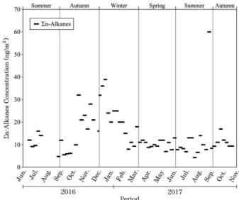
Fig. 4 describes the temporal variation of ∑n-alkanes
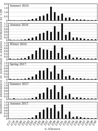
during the study period and the relative abundances of individual n-alkanes normalized by C29, which is one of
the most abundant n-alkanes, are presented in Fig. 5 to visually confirm the distribution profile in each season. Winter 2016 showed the higher average ∑n-alkanes
concentration(21ng/m3) than the other seasons. A few
samples in late autumn of 2016(October-November) and early winter of 2016(December-January) showed relatively elevated ∑n-alkanes concentration; however,
most of the samples had concentrations below 20ng/m3
(overall average of 14ng/m3) during the study period
and the seasonal variation was little. This result suggests that the emission sources, which are not influenced by the seasons, are the dominant inputs for ∑n-alkanes
within the source areas of the sampling site. The highest
∑n-alkanes concentration was observed in late summer
of 2017, when all of the n-alkane homologues appeared at high concentrations. The overall mean concentration of ∑n-alkanes accounted for 0.14% and 0.84% of
PM2.5 and OC, respectively. Also, PM2.5 and OC have
positive correlation with ∑n-alkanes with the Pearson
correlation coefficient(R) of 0.57 and 0.80, respectively.
3.2.3 PAEs
PAEs are widely manufactured as plasticizers to make plastic materials flexible, and also in building materials, food, drinking water, soil, medical devices, cosmetics, children’s toys, and other products(Wang et al., 2017;
Yao et al., 2016; Chou and Wright, 2006). Several
epi-demiological studies have demonstrated that human exposure to PAEs can induce adverse effects, and PAEs are suspected to be endocrine disruptors, which has stimulated public concern(Okamoto et al., 2011; Chou
and Wright, 2006; Duty et al., 2005, 2003). To our
knowledge, there is no previous publication involving the measurement of PAEs in PM2.5 collected from the
ambient atmosphere of Japan.
Measurement values of PAEs in each season are shown in Table 3. The summed concentration of 5 species of PAEs is expressed as ∑PAEs. Fig. 6 presents the
tem-poral variation of ∑PAEs during the study period.
Average ∑PAEs was found to be higher(0.51ng/m3)
in summer 2017 than in other seasons; however, aver-age ∑PAEs in summer 2016(0.26ng/m3) was about
half the summer 2017 value, so there was no clear sea-sonal pattern. One sample in late summer of 2017 showed a relatively high level of ∑PAEs(1.8ng/m3);
however, most of the obtained data were below 1ng/ m3 during the study period and thus no clear seasonal
variation was observed. The reason is uncertain but the
∑PAEs were extremely low in autumn 2017. The
overall mean concentration of ∑PAEs was 0.36ng/
m3, which was one and two orders of magnitude lower
than ∑PAHs and ∑n-alkanes, respectively. Also,
PM2.5 and OC did not indicate correlation with ∑PAEs. Therefore, the target PAEs were not
substan-tially emitted within the source area of the sampling site; however, PAEs those were not measured in this study might be contained in high concentrations in PM2.5, so further research should target these
non-detected compounds.
3.3 Identification of Possible Sources
3.3.1 Diagnostic Ratios of PAHs
The diagnostic ratios of PAHs are a useful tool to identify possible sources and have been developed and applied by many environmental researchers(Wang et al., 2017, 2016; Hayakawa et al., 2016; Zhang et al.,
2016; MikuŠka et al., 2015; Alves et al., 2009; Alves,
2008; Park et al., 2006; Brandenberger et al., 2005;
Yunker et al., 2002; Simcik et al., 1999; Khalili et al.,
Fig. 6. Temporal variation of ΣPAEs concentration.
Fig. 5. Relative abundances of individual n-alkanes normalized by C29 in each season.
1995; Li and Kamens, 1993; Rogge et al., 1993a,
1993b). The compounds involved in each ratio have the same or similar molecular weight, so it may be assumed that they have similar physicochemical prop-erties. Diagnostic ratios vary during different stages of phase transfer and under environmental degradation. In this study, we calculated diagnostic ratios of BeP/ (BeP+BaP), BaA/(BaA +Chr), IP/(IP +BghiP), Fluor/(Fluor+Py), and BghiP/BaP from the mea-sured PAHs shown in Table 2.
Most fresh exhaust emissions typically contain almost the same amount of BeP and BaP. However, BaP more easily degraded than BeP by photochemical reactions in the ambient atmosphere. The atmospheric lifetime of BaP is estimated as ten times shorter than that of BeP(Kalberer et al., 2002). Therefore, the increment of
BeP/(BeP+BaP) can be used as in indicator of the degree of photochemical degradation(i.e., aging) of compounds in the atmospheric environment(Wang et al., 2015; Shen et al., 2013; Alves et al., 2009). The
sea-sonal variation of calculated BeP/(BeP+BaP) in this study ranged from 0.38-0.58. Freshly released BeP/ (BeP+BaP) should have a ratio close to 0.50(MikuŠka
et al., 2015; Park et al., 2006), suggesting that most of
the PM2.5 containing BaP and BeP was emitted from
local or nearby regional sources throughout the study period.
Table 5 presents five different types of developed diagnostic ratios from previous studies and includes BeP/(BeP+BaP), BaA/(BaA +Chr), IP/(IP + BghiP), Fluor/(Fluor+Py), and BghiP/BaP (Hayaka-wa et al., 2016; Wang et al., 2015; Shen et al., 2013;
Alves et al., 2009; Yunker et al., 2002; Simcik et al.,
1999; Khalili et al., 1995; Li and Kamens, 1993; Rogge et al., 1993a, 1993b) and those obtained in this study.
From the comparison of the diagnostic ratios shown in Table 5, most of the diagnostic ratios calculated were Table 5. Comparison of PAHs diagnostic ratios from this study with those reported in previous studies.
Emission sources
Diagnostic ratios
References BeP/(BeP+BaP) (BaABaA/ +Chr) (IP+BghiP)IP/ (FlourFluor/ +Py) BghiP/ BaP
Local emission Index of the aging of particles. Value around 0.5 indicates freshly emitted particles.
Wang et al., 2015; Shen et al., 2013;
Alves et al., 2009
Gasoline 0.17-0.38 0.042-0.22 0.37-0.63 0.34-3.3 Rogge et al., 1993a; Simick et al., 1999;
Khalili et al., 1995; Li and Kamens, 1993
Diesel 0.45-0.64 0.19-0.70 0.20-0.93 0.36-2.2 Yunker et al., 2002; Simick et al., 1999;
Khalili et al., 1995; Rogge et al., 1993a;
Li and Kamens, 1993
Coal 0.35-0.62 0.48-0.85 0.15-1.1 Yunker et al., 2002; Simick et al., 1999
Wood burning 0.36-0.43 0.49-0.77 0.41-0.67 0.64 Yunker et al., 2002; Khalili et al., 1995;
Li and Kamens, 1993
Coke oven 0.34-0.41 0.61 0.90 0.13-0.20 Hayakawa et al., 2016; Simick et al.,
1999; Khalili et al., 1995
Incinerators 1.7-7.1 Simick et al., 1999
Road dust 0.51 0.42 0.91 Yunker et al., 2002; Rogge et al., 1993b
Tire ware 0.17 Rogge et al., 1993b
Brake 0.39 3.5 Rogge et al., 1993b
Range (Average) This study 0.38-0.58 (0.46) 0.29-0.71
(0.43) 0.042-0.56 (0.51) 0.50-0.57 (0.54) 0.52-1.7 (1.1)
Table 6. CPI and Cwax obtained from the measurement results of individual n-alkanes.
Year Season n CPI Cwax (%)
Range Average Range Average 2016 Summer 6 0.73-1.4 1.1 4.3-17 9.0 Autumn 12 1.1-2.0 1.6 12-34 23 Winter 13 1.1-1.6 1.4 9.7-26 19 2017 Spring 13 0.94-3.2 1.7 8.4-53 25 Summer 13 1.2-1.9 1.6 8.9-32 24 Autumn 8 0.95-2.0 1.5 7.7-35 22 Total 65 0.73-3.2 1.5 4.3-53 22
within the range of gasoline, diesel, coal and wood burning emissions. The emissions from gasoline and diesel emissions from vehicles, and coal emissions from industrial sources are not influenced by the seasons, which supports the assumption mentioned above in Section 3.2.1. Therefore, influences of vehicle and industrial emission sources nearby sampling site could be the possible anthropogenic sources of measured PAHs in this study. Kume et al.(2007) have analyzed 21 species of PAHs in suspended particles at urban sites of Shizuoka, Japan, within the area of vehicle and indus-trial emission sources nearby. Their annual means ratios of IP/(IP+BghiP) and BghiP/BaP were 0.51 and 1.28, respectively, which were in good agreement with those obtained in this study.
Moreover, careful consideration of PAHs usage data should be taken in to account when attempting to iden-tify anthropogenic PAHs sources because PAHs can be emitted from various source types. Therefore, other molecular markers and/or tracers should be gathered for more accurate source apportionment.
3.3.2 Historical Distribution, CPI and Cwax of
n-Alkanes
Table 3 and Fig. 5 indicate that C23-C33 were the
main homologues contributing to the ∑n-alkanes.
Previous research has shown that carbon number with a strong predominance of odd carbon number indi-cates a significant contribution from biogenic contribu-tors(Rogge et al., 1993c), whose abundances of odd
carbon number higher than 24 are approximately one magnitude higher than those of even carbon number. Whereas n-alkanes released from fossil fuel sources do not show such predominant tendency(Alves et al.,
2009; Simoneit et al., 1991). Fig. 5 shows that
odd-numbered carbon homologues were not dominant dur-ing the study period. Therefore, contributions arisdur-ing from anthropogenic inputs might have been higher than biogenic inputs at the study site.
For the further interpretation of obtained data associ-ated with n-alkanes, we used the carbon preference index (CPI) and contribution of plant wax to n-alkanes(Cwax)
to assess the variability of sources, and they are listed in Table 6. The CPI can be used to distinguish biogenic and anthropogenic inputs. It is defined as the sum of the concentrations of the odd carbon number n-alkanes (∑Codd) divided by the sum of the concentrations of
the even carbon number n-alkanes(∑Ceven), which was
calculated as follows:
∑Codd ∑(C17 to C39)
CPI=---=--- (1) ∑Ceven ∑(C18 to C40)
Plant wax n-alkanes exhibit a strong odd carbon num-ber predominance and thus increase the CPI value(Park
et al., 2006). Conversely, anthropogenic inputs such as
fossil fuels reduce the CPI value. The CPI typical values in the urban environment range from 1.1 to 2.0, while a CPI higher than 2.0 has a stronger biogenic influence (Alves et al., 2009). In the present study, the CPI values
during the study period were in the range 0.73-3.2 with an average of 1.5, as shown in Table 6. A CPI value above 2.0 was observed just in one sample in spring 2017 (CPI=3.2, for 2-10 May), suggesting that most of the measured n-alkanes during the study period were anth-ropogenic in origin.
Another methodology to analyze the contribution of plant wax sources to n-alkanes can be expressed through Cwax(Wang et al., 2015; Yadav et al., 2013; Alves, 2008;
Park et al., 2006; Simoneit et al., 1991). Cwax gives the percentage concentration input of wax n-alkanes from biogenic sources in sample. The Cwax is calculated as
follows: (Cn-1+Cn+1) ∑
{
Cn- ---}
2 Cwax=--- ×100 (2) ∑n·Alkaneswhere n is the odd number of analyzed n-alkanes. Mea-sured Cn values below the LOD were replaced with the
value of LOD/2, and the negative values of {Cn-(Cn-1
+Cn+1)/2} were determined as zero. Table 6 shows
that the percentages of Cwax were in the range of
4.3-53% with an average of 22%. The higher percentage values indicate greater contributions from biogenic sources(Wang et al., 2015). The highest Cwax value of 53% was calculated from the same sample as CPI = 3.2, which could possibly mean that the contribution of biogenic sources was larger than sample during the period of 2-10 May 2017. Comprehensive evaluation including the historical distributions of n-alkanes homologues, CPI, and Cwax, indicates that the observed
n-alkanes may largely originate from anthropogenic sources for most of the samples in this study. Further identification of the emission sources of n-alkanes in PM2.5 will be conducted in future research.
4. SUMMARY AND CONCLUSIONS
A long time series(approximately 17 months) of quan-titative data of non-polar organic compounds constitut-ing PM2.5 was created from samples collected at Ichihara,
one of the largest industrial areas in Japan. Sample collec-tion and analysis took place continuously from June 2016 to October 2017. The target non-polar organic compounds were 21 species of PAHs, 24 species of n-alkanes, and 5 species of PAHs, and these were simul-taneously measured using GC/MS. The results indicate that anthropogenic sources were the dominant inputs for the most PAHs and n-alkanes throughout the study peri-od. Identification of the emission sources of individual organic compounds in PM2.5 will be conducted in future
research. To our knowledge, this paper describes the first attempt to measure such a large number of different non-polar organic compounds in PM2.5 from the ambient
atmosphere of Japan to create a long time series. The findings will provide valuable data and information to environmental researchers. The main findings are as fol-lows:
(1) The average concentrations of ∑PAHs, ∑n-alkanes, and ∑PAEs in each season remained
nearly level(except for a few high ∑PAHs in early
win-ter and ∑n-alkanes in late autumn and early winter),
and no strong seasonal variations were observed thr-oughout the study period. These results suggest that the emission sources, which are not influenced by the sea-sons, are the dominant inputs for the target organic com-pounds.
(2) The contributions of ∑PAHs, ∑n-alkanes, and ∑PAEs to the PM2.5 mass concentration were each less
than 1%.
(3) The target PAEs were not substantially emitted within the source area of the sampling site.
(4) All of the calculated BeP/(BeP+BaP) ratios were close to 0.50, which indicates that PM2.5
contain-ing BaP and BeP were emitted from local or nearby regional anthropogenic sources throughout the study period.
(5) From the analysis of diagnostic ratios, gasoline, diesel and coal emissions could be possible anthropo-genic sources of measured PAHs in this study.
(6) The distributions of n-alkane homologues and calculated results of CPI and Cwax, indicate that
n-alkanes at the study site may largely originate from anthropogenic sources. Further identification of the
emission sources of n-alkanes in PM2.5 will be
conduct-ed in future research.
REFERENCES
Ahmed, M., Guo, X., Zhao, X.M.(2016) Determination and
analysis of trace metals and surfactant in air particulate matter during biomass burning haze episode in Malaysia. Atmospheric Environment 141, 219-229.
Alves, C.A.(2008) Characterisation of solvent extractable
organic constituents in atmospheric particulate matter: an overview. Anais da Academia Brasileira de Ciências 80, 21-82.
Alves, C.A., Vicente, A., Evtyugina, M., Pio, C.A., Hoffer, A.,
Kiss, G., Decesari, S., Hillamo, R., Swietlicki, E.(2009)
Characterisation of Hydrocarbons in Atmospheric Aero-sols from Different European Sites. International Journal of Environmental and Ecological Engineering 3, 263-269. Alves, N.O., Brito, J., Caumo, S., Arana, A., Hacon, S.S., Artaxo,
P., Hillamo, P., Teinilä, K., Medeiros, S.R.B., Vasconcellos,
P.C.(2015) Biomass burning in the Amazon region: Aerosol
source apportionment and associated health risk assessment. Atmospheric Environment 120, 277-285.
Brandenberger, S., Mohr, M., Grob, K., Neukomb, H.P.(2005)
Contribution of unburned lubricating oil and diesel fuel to particulate emission from passenger cars. Atmospheric Envi-ronment 39, 6985-6994.
Chou, K., Wright, R.O.(2006) Phthalates in food and medical
devices. Journal of Medical Toxicology 2, 126-135.
Chow, J.C., Watson, J.G., Pritchett, L.C., Pierson, W.R., Frazier,
C.A., Purcell, R.G.(1993) The DRI thermal/optical
reflec-tance carbon analysis system: description, evaluation and applications in U.S. air quality studies. Atmospheric Envi-ronment 27, 1185-1201.
Chow, J.C., Watson, J.G., Crow, D., Lowenthal, D.H., Merrifield,
T.Y.A.(2001) Comparison of IMPROVE and NIOSH
car-bon measurements. Aerosol Science and Technology 34, 23-34.
Duty, S.M., Silva, M.J., Barr, D.B., Brock, J.W., Ryan, L., Chen,
Z., Herrick, R.F., Christiani, D.C., Hauser, R.(2003)
Phthal-ate exposure and human semen parameters. Epidemiology 14, 269-277.
Duty, S.M., Calafat, A.M., Silva, M.J., Ryan, L., Hauser, R. (2005) Phthalate exposure and reproductive hormones in adult men. Human Reproduction 20, 604-610.
EU(2004) Directive 2004/107/EC of the European
parlia-ment and of the council of 15 December 2004 relating to arsenic, cadmium, mercury, nickel and polycyclic aromatic hydrocarbons in ambient air. http://eur-lex.europa.eu/ LexUriServ/LexUriServ.do?uri=OJ:L:2005:023:0003:001
6:EN:PDF.(Accessed on February 5 , 2018)
Fuzzi, S., Baltensperger, U., Carslaw, K., Decesari, S., Gon, H.D., Facchini, M.C., Fowler, D., Koren, I., Langford, B., Lohm-ann, U., Nemitz, E., Pandis, S., Riipinen, I., Rudich, Y., Schaap, M., Slowik, J.G., Spracklen, D.V., Vignati, E., Wild,
M., Williams, M., Gilardoni, S.(2015) Particulate matter, air quality and climate: lessons learned and future needs. Atmo-spheric Chemistry and Physics 15, 8217-8299.
Hayakawa, K., Tang, N., Morisaki, H., Toriba, A., Akutagawa,
T., Sakai, S.(2016) Atmospheric polycyclic and
nitropoly-cyclic aromatic hydrocarbons in an iron-manufacturing city. Asian Journal of Atmospheric Environment 10, 90-98. He, L.Y., Hu, M., Huang, X.F., Yu, B.D., Zhang, Y.H., Liu, D.Q. (2004) Measurement of emissions of fine particulate organic matter from Chinese cooking. Atmospheric Envi-ronment 38, 6557-6564.
IARC(2010) IARC monographs on the evaluation of
carcino-genic risks to humans. Volume 92. Some non-heterocyclic polycyclic aromatic hydrocarbons and some related expo-sures.
IARC(2012) IARC monographs on evaluation of
carcino-genic risks to humans. Chemical agents and related occu-pations. Volume 100F. A review of human carcinogens. Ichikawa, Y., Watanabe, T., Horimoto, Y., Ishii, K., Naito, S.
(2017) Organic components of PM2.5 observed in Chiba
Prefecture during the fiscal years 2014-2016. Journal of
Environmental Laboratories Association 42, 60-67.
(writ-ten in Japanese with English abstract, figures and tables).
Ichikawa, Y., Naito, S., Ishii, K., Oohashi, H.(2015) Seasonal
variation of PM2.5 components observed in an industrial
area of Chiba Prefecture, Japan. Asian Journal of Atmo-spheric Environment 9, 66-77.
IPCC(2013) Climate change 2013. The physical science basis.
Summary for policymakers, technical summary and fre-quently asked questions. Contribution of working group I to the fifth assessment report of the intergovernmental panel on climate change. Cambridge University Press, United Kingdom and New York.
Jacob, D.J.(1999) Introduction to atmospheric chemistry.
Princeton University Press, New Jersey, pp. 148-154. Kakimoto, H., Matsumoto, Y., Sakai, S., Kanoh, F., Arashidani,
K., Tang, N., Akutsu, K., Nakajima, A., Awata, Y., Toriba, A.,
Kizu, R., Hayakawa, K.(2002) Comparison of atmospheric
polycyclic aromatic hydrocarbons and nitropolycyclic
aro-matic hydrocarbons in an industrialized city(Kitakyushu)
and two commercial cities(Sapporo and Tokyo). Journal of
Health Science 48, 370-375.
Kalberer, M., Henne, S., Prevot, A.S.H., Steinbacher, M. (2004) Vertical transport and degradation of polycyclic aromatic hydrocarbons in an Alpine Valley. Atmospheric Environment 38, 6447-6456.
Kawamura, K., Bikkina, S.(2016) A review of dicarboxylic acids
and related compounds in atmospheric aerosols: molecular distributions, sources and transformation. Atmospheric Research 170, 140-160.
Khalili, N.R., Scheff, P.A., Holsen, T.M.(1995) PAH source
fin-gerprints for coke ovens, diesel and, gasoline engines, high-way tunnels, and wood combustion emissions. Atmospheric Environment 29, 533-542.
Kume, K., Ohura, T., Noda, T., Amagai, T., Fusaya, M.(2007)
Seasonal and spatial trends of suspended-particle associat-ed polycyclic aromatic hydrocarbons in urban Shizuoka, Japan. Journal of Hazardous Materials 144, 513-521.
Li, C.K., Kamens, R.M.(1993) The use of polycyclic
aromat-ic hydrocarbons as source signatures in receptor modeling. Atmospheric Environment 27A, 523-532.
Li, X., Chen, M., Le, H.P., Wang, F., Guo, Z., Iinuma, Y., Chen,
J., Herrmann, H.(2016) Atmospheric outflow of PM2.5
sac-charides from megacity Shanghai to East China Sea: Impact of biological and biomass burning sources. Atmospheric Environment 143, 1-14.
Mikuška, P., Křůmal, K., Večeřa, Z.(2015) Characterization
of organic compounds in the PMF aerosols in winter in an
industrial urban area. Atmospheric Environment 105, 97-108.
Mikuška, P., Kubátková, N., Křůmal, K., Večeřa, Z.(2017)
Seasonal variability of monosaccharide anhydrides, resin
acids, methoxyphenols and saccharides in PM2.5 in Brno,
the Czech Republic. Atmospheric Pollution Research 8, 576-586.
Okamoto, Y., Ueda, K., Kojima, N.(2011) Potential risks of
phthalate esters: acquisition of endocrine-disrupting activ-ity during environmental and metabolic processing. Jour-nal of Health Science 57, 497-503.
Oros, D.R., Standley, L.J., Chen, X., Simoneit, B.R.T.(1999)
Epicuticular wax compositions of predominant conifers of Western North America. Zeitschrift für Naturforschung C 54, 17-24.
Park, S.S., Bae, M.S., Schauer, J.J., Kim, Y.J., Cho, S.Y., Kim, S.J.
(2006) Molecular composition of PM2.5 organic aerosol
measured at an urban site of Korea during the ACE-Asia campaign. Atmospheric Environment 40, 4182-4198. Rogge, W.F., Hildemann, L.M., Mazurek, M.A., Cass, G.R.,
Simoneit, B.R.T.(1993a) Sources of fine organic aerosol. 2.
Noncatalyst and catalyst-equipped automobiles and heavy-duty diesel trucks. Environmental Science and Technology 27, 636-651.
Rogge, W.F., Hildemann, L.M., Mazurek, M.A., Cass, G.R.,
Simoneit, B.R.T.(1993b) Sources of fine organic aerosol. 3.
Road dust, tire debris, and organometallic brake lining dust: roads as sources and sinks. Environmental Science and Technology 27, 1892-1904.
Rogge, W.F., Hildemann, L.M., Mazurek, M.A., Cass, G.R.,
Simoneit, B.R.T.(1993c) Sources of fine organic aerosol. 4.
Particulate abrasion products from leaf surfaces of urban plants. Environmental Science and Technology 27, 2700-2711.
Schwartz, J., Neas, L.M.(2000) Fine particles are more strongly
associated than coarse particles with acute respiratory health effects in schoolchildren. Epidemiology 11, 6-10.
Shen, G., Tao, S., Wei, S., Zhang, Y., Wang, R., Wang, B., Li, W., Shen, H., Huang, Y., Chen, Y., Chen, H., Yang, Y., Wang, W.,
Wang, X., Liu, W., Staci, L.M. Simonich, S.L.M.(2012)
Emissions of Parent, Nitro, and Oxygenated Polycyclic Aro-matic Hydrocarbons from Residential Wood Combustion in Rural China. Environmental Science and Technology 46, 8123-8130.
Simcik, M.F., Eisenreich, S.J., Lioy, P.J.(1999) Source
appor-tionment and source/sink relationships of PAHs in the coa-stal atmosphere of Chicago and Lake Michigan. Atmospher-ic Environment 33, 5071-5078.
Simoneit, B.R.T., Sheng, G., Chen, X., Fu, J., Zhang, J., Xu, Y. (1991) Molecular marker study of extractable organic mat-ter in aerosols from urban areas of China. Atmospheric Environment 25A, 2111-2129.
Simoneit, B.R.T., Kobayashi, M., Mochida M., Kawamura, K.,
Lee, M., Lim, H.J. Turpin, B.J., Komazaki, Y.(2004)
Com-position and major sources of organic compounds of aero-sol particulate matter sampled during the ACE-Asia cam-paign. Journal of Geophysical Research 109, D19S10.
Simoneit, B.R.T.(2002) Biomass burning - a review of organic
tracers for smoke from incomplete combustion. Applied Geochemistry 17, 129-162.
Simoneit, B.R.T., Sheng, G., Chen, X., Fu, J., Zhang, J., Xu, Y. (1991) Molecular marker study of extractable organic mat-ter in aerosols from urban areas of China. Atmospheric Environment 25A, 2111-2129.
Suzuki, G., Morikawa, T., Kashiwakura, K., Tang, N., Toriba,
A., Hayakawa, K.(2015) Variation of polycyclic aromatic
hydrocarbons and nitropolycyclic aromatic hydrocarbons in airborne particulates collected in Japanese capital area. Journal of Japan Society for Atmospheric Environment 50,
117-122.(written in Japanese with English abstract, figures
and tables)
Ueda, K.(2011) The health effects of fine particulate matter:
Evidence among Japanese populations and trends in epide-miological studies. Journal of Japan Society for
Atmo-spheric Environment 46, A7-A13.(in Japanese)
Wang, J., Ho, S.S., Cao, J., Huang, R., Zhou, J., Zhao, Y., Xu,
H., Liu, S., Wang, G., Shen, Z., Han, Y.(2015)
Characteris-tics and major sources of carbonaceous aerosols in PM2.5
from Sanya, China. Science of The Total Environment 530-531, 110-119.
Wang, J., Ho, S.S., Ma, S., Cao, J., Dai, W., Liu, S., Shen, Z.,
Huang, R., Wang, G., Han, Y.(2016) Characterization of
PM2.5 in Guangzhou, China: uses of organic markers for
supporting source apportionment. Science of The Total Environment 550, 961-971.
Wang, J., Guinot, B., Dong, Z., Li, X., Xu, H., Xiao, S., Ho,
S.S.H., Liu, S., Cao, J.(2017) PM2.5-bound polycyclic
aro-matic hydrocarbons(PAHs), oxygenated-PAHs and
phthal-ate esters(PAEs) inside and outside middle school
class-rooms in Xi’an, China: concentration, characteristics and health risk assessment. Aerosol and Air Quality Research 17, 1811-1824.
WHO(2013) Review of evidence on health aspects of air
pol-lution - RVIHAAP Project. World Health Organization regional office for Europe, Copenhagen.
Yao, H.Y., Han, Y., Gao, H., Huang, K., Ge, X., Xu, Y.Y., Xu, Y.Q., Jin, Z.X., Sheng, J., Yan, S.Q., Zhu, P., Hao, J.H., Tao,
F.B.(2016) Maternal phthalate exposure during the first
trimester and serum thyroid hormones in pregnant women and their newborns. Chemosphere 157, 42-48.
Yadav, S., Tandon, A., Attri, A.K.(2013) Monthly and
season-al variations in aerosol associated n-season-alkane profiles in rela-tion to meteorological parameters in New Delhi, India. Aerosol and Air Quality Research 13, 287-300.
Yang, F., Kawamura, K., Chen, J., Ho, K., Lee, S., Gao, Y., Cui,
L., Wang, T., Fu, P.(2016) Anthropogenic and biogenic
organic compounds in summertime fine aerosols(PM2.5)
in Beijing, China. Atmospheric Environment 124, 166-175.
Yunkera, M.B., Macdonald, R.W., Vingarzan, R., Mitchell, R.H.,
Goyette, D., Sylvestre, S.(2002) PAHs in the Fraser River
basin: a critical appraisal of PAH ratios as indicators of PAH source and composition. Organic Geochemistry 33, 489-515.
Zhang, M., Xie, J., Wang, Z., Zhao, L., Zhang, H., Li, M.(2016)
Determination and source identification of priority
polycy-clic aromatic hydrocarbons in PM2.5 in Taiyuan, China.
Atmospheric Research 178-179, 401-414.
Zhang, Y., Obrist, D., Zielinska, B., Gertler, A.(2013)
Particu-late emissions from different types of biomass burning. Atmospheric Environment 72, 27-35.