Advanced Thermodynamics (M2794.007900)

Consequences of the First Law

Chapter 5

Advanced Thermodynamics (M2794.007900)

Min Soo Kim

Seoul National University

A.1 Partial Derivatives

Consider a function of three variables, 𝑓 𝑥, 𝑦, 𝑧 = 0

since only two variables are independent, we can write 𝑥 = 𝑥 𝑦, 𝑧 , 𝑦 = 𝑦 𝑥, 𝑧

Then d𝑥 = ( ^𝜕𝑥

𝜕𝑦 )_𝑧𝑑𝑦 + (^𝜕𝑥

𝜕𝑧 )_𝑦𝑑𝑧, and d𝑦 = ( ^𝜕𝑦

𝜕𝑥 )_𝑧𝑑𝑥 + ( ^𝜕𝑦

𝜕𝑧 )_𝑥𝑑𝑧 We obtain,

d𝑥 = ( ^𝜕𝑥

𝜕𝑦 )_𝑧 ( ^𝜕𝑦

𝜕𝑥 )_𝑧𝑑𝑥 + ( ^𝜕𝑦

𝜕𝑧 )_𝑥𝑑𝑧 + ( ^𝜕𝑥

𝜕𝑧 )_𝑦𝑑𝑧

A.1 Partial Derivatives

d𝑥 = ( ^𝜕𝑥

𝜕𝑦 )_𝑧 ( ^𝜕𝑦

𝜕𝑥 )_𝑧𝑑𝑥 + ( ^𝜕𝑦

𝜕𝑧 )_𝑥𝑑𝑧 + ( ^𝜕𝑥

𝜕𝑧 )_𝑦𝑑𝑧

= ( ^𝜕𝑥

𝜕𝑦 )_𝑧( ^𝜕𝑦

𝜕𝑥 )_𝑧𝑑𝑥 + ( ^𝜕𝑥

𝜕𝑦 )_𝑧( ^𝜕𝑦

𝜕𝑧 )_𝑥 + ( ^𝜕𝑥

𝜕𝑧 )_𝑦 𝑑𝑧 If d𝑧 = 0 and d𝑥 ≠ 0 ,

𝝏𝒙

𝝏𝒚 𝒛 = _𝝏𝒚^𝟏

𝝏𝒙 𝒛

. This expression is known as the reciprocal relation.

If d𝑥 = 0 and d𝑧 ≠ 0 ,

𝜕𝑥

𝜕𝑦 𝑧

𝜕𝑦

𝜕𝑧 𝑥 = − ^𝜕𝑥

𝜕𝑧 𝑦

A.1 Partial Derivatives

𝜕𝑥

𝜕𝑦 𝑧

𝜕𝑦

𝜕𝑧 𝑥 = − ^𝜕𝑥

𝜕𝑧 𝑦 (previous slide)

𝜕𝑥

𝜕𝑧 𝑦 = _𝜕𝑧¹

𝜕𝑥 𝑦

(using reciprocal relation)

Substituting these equations yield,

𝝏𝒙

𝝏𝒚 𝒛

𝝏𝒚

𝝏𝒛 𝒙

𝝏𝒛

𝝏𝒙 𝒚 = −𝟏. The cyclical rule, or cyclical relation.

A.1 Partial Derivatives

Consider a function 𝑢 of three variables x, y, z can be written as a function of only two variables and those two variables are independent.

𝑢 = 𝑢 𝑥, 𝑦 Alternatively,

𝑥 = 𝑥 𝑢, 𝑦 Then

d𝑥 = ^𝜕𝑥

𝜕𝑢 𝑦 𝑑𝑢 + ^𝜕𝑥

𝜕𝑦 𝑢 𝑑𝑦.

If we divide the equation by d𝑧 while holding 𝑢 constant,

𝜕𝑥

𝜕𝑧 𝑢 = ^𝜕𝑥

𝜕𝑦 𝑢

𝜕𝑦

𝜕𝑧 𝑢. The chain rule of differentiation.

5.1 The Gay-Lussac-Joule Experiment

In general,

𝑢 = 𝑢 𝑇, 𝑣

using the cyclical and reciprocal relations,

(

𝜕𝑣

)

= −

𝜕𝑢

𝜕𝑣 )_𝑇 (^𝜕𝑢

𝜕𝑇)_𝑣

for a reversible process,

𝑐

= (

𝜕𝑇

)

∴ (

𝜕𝑣

)

= −𝑐

(

𝜕𝑣

)

Then how can we keep

𝑢

5.1 The Gay-Lussac-Joule Experiment

𝑑𝑢 = 𝛿𝑞 − 𝛿𝑤 ⇒ free expansion

𝑇

= 𝑇

+ ׬

0

𝑣₁

(

𝜕𝑣

)

𝑑𝑣, 𝜂 ≡

𝜕𝑣 )_𝑢 : Joule’s coefficient From Joule’s experimental result,

𝜂 = ^𝜕𝑇

𝜕𝑣 𝑢 < 0.001 K kilomole m⁻³

𝒗_𝟎 , 𝑻_𝟎 𝒗_𝟏 − 𝒗_𝟎

thermal insulation gas

sample

diaphragm

vacuum

= 0 (adiabatic)

= 0 (no work)

5.1 The Gay-Lussac-Joule Experiment

for a Van der Waals gas, (Problem 5-3)

𝜂 = − 𝑎 𝑣

𝑐

for an ideal gas,

by using the equation

𝑑𝑢 = 𝑇𝑑𝑠 − 𝑃𝑑𝑣

𝜕𝑢

𝜕𝑣 𝑇

= 𝑇

𝜕𝑣 𝑇

− 𝑃 = 𝑇

𝜕𝑇 𝑣

− 𝑃 = 𝑇 [

𝜕𝑇

𝑅𝑇

𝑣

]

− 𝑃

=

𝑣

− 𝑃 = 0

Then 𝑢 = 𝑢(𝑇)

5.1 The Gay-Lussac-Joule Experiment

for a real gas,

by using the equation

𝑑𝑞 =

𝜕𝑇 𝑣

𝑑𝑇 +

𝜕𝑣 𝑇

+ 𝑃 𝑑𝑣

𝑑𝑞

𝑇

=

𝑇

𝜕𝑢

𝜕𝑇 𝑣

𝑑𝑇 +

𝑇

𝜕𝑢

𝜕𝑣 𝑇

+ 𝑃 𝑑𝑣

𝜕

𝜕𝑣 1 𝑇

𝜕𝑢

𝜕𝑇

=

𝜕𝑇 1 𝑇

𝜕𝑢

𝜕𝑣

+ 𝑃

1 𝑇

𝜕²𝑢

𝜕𝑣𝜕𝑇

= −

𝑇²

𝜕𝑢

𝜕𝑣

+ 𝑃 +

𝑇

𝜕²𝑢

𝜕𝑣𝜕𝑇

+

𝑇

𝜕𝑃

𝜕𝑇

𝜕𝑢

𝜕𝑣 𝑇

= 𝑇

𝜕𝑇 𝑣

− 𝑃

5.2 The Joule-Thomson Experiment

Since the process takes place in an insulated cylinder,

δ𝑞 = 0

specific work done in forcing the gas through the plug, 𝑤₁ = ׬_𝑣

1

0 𝑃₁ 𝑑𝑣 = −𝑃₁𝑣₁ specific work done by the gas in the expansion, 𝑤₂ = ׬₀^𝑣2𝑃₂ 𝑑𝑣 = 𝑃₂ 𝑣₂

Porous plug

Initial state Final state

𝑷_𝟏, 𝒗_𝟏 , 𝑻_𝟏 𝑷_𝟐, 𝒗_𝟐 , 𝑻_𝟐

5.2 The Joule-Thomson experiment

The total work, 𝑤 = 𝑤₁ + 𝑤₂ = 𝑃₂ 𝑣₂ − 𝑃₁ 𝑣₁ = 𝑢₁ − 𝑢₂ 𝑢₁ + 𝑃₁ 𝑣₁ = 𝑢₂ + 𝑃₂ 𝑣₂ ⟺ ℎ₁ = ℎ₂

Thus, a throttling process occurs at constant enthalpy.

constant

5.2 The Joule-Thomson experiment

Joule-Thomson coefficient

𝜇

≡ (

𝜕𝑃

)

the point where 𝜇_𝐽𝑇 = 0 is called inversion point.

from ℎ = ℎ 𝑇, 𝑃 , 𝑑ℎ = ( ^𝜕ℎ

𝜕𝑇 )_𝑃 𝑑𝑇 + ( ^𝜕ℎ

𝜕𝑃 )_𝑇 𝑑𝑃 𝜇_𝐽𝑇 ≡ ( ^𝜕𝑇

𝜕𝑃 )_ℎ = ^{𝑇2−𝑇1}

𝑃₂−𝑃₁ ℎ

𝑇₂ = 𝑇₁ − 𝜇 𝑃₂ − 𝑃₁

The gas is cooling when the 𝜇 is positive and heating when the 𝜇 is negative

5.2 The Joule-Thomson experiment

Joule-Thomson coefficient

𝜇

=

𝜕𝑃 ℎ

= −

𝜕ℎ 𝑃

𝜕ℎ

𝜕𝑃 𝑇

=

𝐶_𝑃

𝑇

𝜕𝑇 𝑃

− 𝑣

for an ideal gas, 𝜇_𝐽𝑇 = 0,

𝜕ℎ

𝜕𝑃 𝑇 = 0 and ℎ = ℎ 𝑇 for a Van der Waals gas, 𝑃 = ^𝑅𝑇

𝑣−𝑏 − ^𝑎

𝑣²

𝜇

= 1 𝑐

2𝑎

𝑅𝑇 1 − 𝑏 𝑣

2

− 𝑏 1 − 2𝑎

𝑣𝑅𝑇 1 − 𝑏 𝑣

2

If 𝜇_𝐽𝑇 = 0,

𝑇

=

𝑏𝑅

1 −

𝑣 2

5.3 Heat engines and the Carnot cycle

Carnot cycle

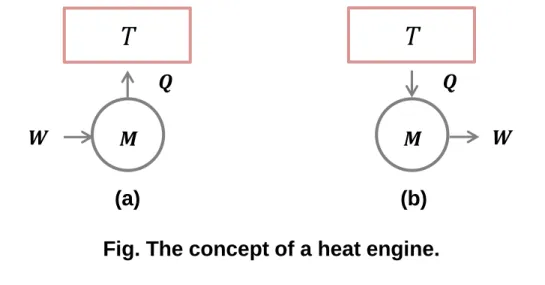
In (a), work is done on the system and is converted to heat.

In (b), heat is extracted from a reservoir and is converted to mechanical work.

This configuration is not possible.

𝑇

𝑸

𝑾 𝑴

𝑇

𝑸 𝑴 𝑾

(a) (b)

Fig. The concept of a heat engine.

5.3 Heat engines and the Carnot cycle

Carnot cycle

Can the work done by the system be equal to the heat in?

The second law of thermodynamics states unequivocally that it is impossible to construct a perfect heat engine.

𝑇

𝑸 𝑴 𝑾

(b) (c)

Fig. The concept of a heat engine.

𝑇_𝑏

𝑇_𝑎

𝑸_𝑯

𝑸_𝑳 𝑴 𝑾

5.3 Heat engines and the Carnot cycle

Clausius statement

It is impossible to construct a device that operates in a cycle and whose sole effect is to transfer heat from a cooler body to a hotter body.

Kelvin-Planck statement

It is impossible to construct a device that operates in a cycle and produces no other effect than the performance of work and the exchange of heat with a single reservoir.

5.3 Heat engines and the Carnot cycle

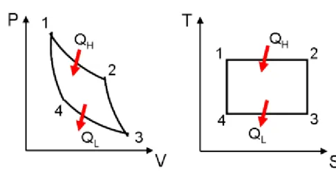
Carnot cycle

1 – 2 : isothermal expansion 2 – 3 : adiabatic expansion 3 – 4 : isothermal compression 4 – 1 : adiabatic compression 𝑇_𝑏

𝑇_𝑎

𝑸_𝑯

𝑸_𝑳

𝑾

Fig. P-V and T-S diagrams of Carnot cycle.

5.3 Heat engines and the Carnot cycle

The efficiency of the engine, 𝜂 = 𝑊

𝑄_𝐻 = 𝑊

𝑄_𝐻 = output input Applying the first law to the system,

∆𝑈 = 𝑄_𝐻 + 𝑄_𝐿 − 𝑊 = 𝑄_𝐻 − 𝑄_𝐿 − 𝑊

Since the system is in a cyclical process, ∆𝑈 = 0. Then, 𝑊 = 𝑄_𝐻 + 𝑄_𝐿 or 𝑊 = 𝑄_𝐻 − 𝑄_𝐿

Substituting the equations,

𝜂 =

𝑄_𝐻

= 1 +

𝑄_𝐻

= 1 −

𝑄_𝐻

5.3 Heat engines and the Carnot cycle

for an ideal gas, 𝑃𝑣 = 𝑅𝑇 , 𝑢 = 𝑢 𝑇 ,

for isothermal process, 𝑄_𝐻 = 𝑊₁₂ = 𝑛 ത𝑅 𝑇_𝑏 ln^𝑉2

𝑉₁

𝑄_𝐿 = 𝑊₃₄ = 𝑛 ത𝑅 𝑇_𝑎 ln^𝑉4

𝑉₃

⇒ ^𝑄𝐻

𝑄_𝐿 = −^𝑇𝑏

𝑇_𝑎

for adiabatic process, 𝑃𝑉^𝛾 = 𝑐𝑜𝑛𝑠𝑡𝑎𝑛𝑡 , 𝑇_𝑏 𝑉₂^𝛾−1 = 𝑇_𝑎 𝑉₃^𝛾−1

𝑇_𝑏 𝑉₁^𝛾−1 = 𝑇_𝑎 𝑉₄^𝛾−1

⇒ ^𝑉2

𝑉₁ = ^𝑉3

𝑉₄

The efficiency of the Carnot cycle, 𝜂 = 1 + ^𝑄𝐿

𝑄_𝐻 = 1 − ^𝑇𝑎

𝑇_𝑏

𝑠₂ − 𝑠₁ = 𝑐_𝑣ln𝑇₂

𝑇₁ + 𝑅ln𝑣₂ 𝑣₁

= 𝑐_𝑝ln𝑇₂

𝑇₁ − 𝑅ln𝑃₂

𝑃₁ = 0 𝑐_𝑣 = 1

𝜅 − 1𝑅, 𝑐_𝑝 = 𝜅 𝜅 − 1𝑅 𝑃₂

𝑃₁ = 𝑣₂ 𝑣₁

𝜅

5.3 Heat engines and the Carnot cycle

Carnot engine has the maximum efficiency for any engine that one might design.

1. Carnot engine operates between two reservoirs and that it is reversible.

2. If a working substance other than an ideal gas is used, the shape of curves in the P-V diagram will be difference.

3. The efficiency would be 100 percent if we were able to obtain a low temperature reservoir at absolute zero. →However this is forbidden by the third law.

5.3 Heat engines and the Carnot cycle

Carnot refrigerator

Reverse process of Carnot engine Coefficient of performance(COP)

COP ≡ − 𝑄

𝑊 = 𝑄

𝑊 = 𝑄

𝑄

− 𝑄

= 𝑇

𝑇

− 𝑇

We introduce a minus sign in order to make the COP a positive quantity :

The heat 𝑄_𝐿 is extracted from the low temperature reservoir and W is the work done on the system. 𝑄_𝐿 is positive (heat flow into the system) and W is negative (work done on the system)

𝑇_𝑏

𝑇_𝑎

𝑸_𝑯

𝑸_𝑳

𝑾

5.3 Heat engines and the Carnot cycle

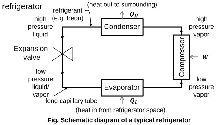
Typical refrigerator

1. The refrigerant is a substance chosen to be a saturated liquid at the pressure and temperature of condenser.

2. The liquid undergoes a throttling process in which it is cooled and is partially

Condenser

Evaporator 𝑸_𝑯

𝑸_𝑳

𝑾

Compressor

Expansion valve

low pressure

liquid/

vapor

low pressure

vapor high pressure

vapor high

pressure liquid

(heat out to surrounding)

(heat in from refrigerator space) refrigerant

(e.g. freon)

long capillary tube

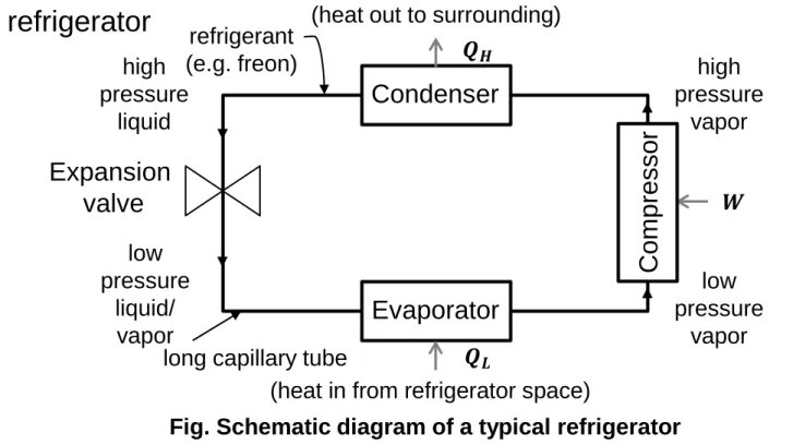
Fig. Schematic diagram of a typical refrigerator

5.3 Heat engines and the Carnot cycle

Condenser

Evaporator 𝑸_𝑯

𝑸_𝑳

𝑾

Compressor

Expansion valve

low pressure

liquid/

vapor

low pressure

vapor high pressure

vapor high

pressure liquid

(heat out to surrounding)

(heat in from refrigerator space) refrigerant

(e.g. freon)

long capillary tube

Fig. Schematic diagram of a typical refrigerator

Typical refrigerator

3. The vaporization is completed in the evaporator: the heat is absorbed by the refrigerant from the low temperature reservoir (the interior refrigerator space).

4. The low pressure vapor is then adiabatically compressed and isobarically cooled

5.3 Heat engines and the Carnot cycle

Typical refrigerator

Refrigerator are designed to extract as much heat as possible from a cold reservoir with small expenditure of work.

The coefficient of performance of a household refrigerator is in the range of 5 to 10.