저작자표시-비영리-변경금지 2.0 대한민국 이용자는 아래의 조건을 따르는 경우에 한하여 자유롭게
l 이 저작물을 복제, 배포, 전송, 전시, 공연 및 방송할 수 있습니다. 다음과 같은 조건을 따라야 합니다:
l 귀하는, 이 저작물의 재이용이나 배포의 경우, 이 저작물에 적용된 이용허락조건 을 명확하게 나타내어야 합니다.
l 저작권자로부터 별도의 허가를 받으면 이러한 조건들은 적용되지 않습니다.
저작권법에 따른 이용자의 권리는 위의 내용에 의하여 영향을 받지 않습니다. 이것은 이용허락규약(Legal Code)을 이해하기 쉽게 요약한 것입니다.
Disclaimer
저작자표시. 귀하는 원저작자를 표시하여야 합니다.
비영리. 귀하는 이 저작물을 영리 목적으로 이용할 수 없습니다.
변경금지. 귀하는 이 저작물을 개작, 변형 또는 가공할 수 없습니다.
i
공학박사 학위논문
Modelling of Liquid Film Off-take in Reactor Vessel Upper Downcomer Based on
High-fidelity Experiment and Simulation
고정밀 실험 및 해석에 기반한
원자로 강수부 상부에서의 액막 견인 모델링
2021 년 8 월
서울대학교 대학원 에너지시스템공학부
최 치 진
ii
i
Abstract
Modelling of Liquid Film Off-take in Reactor Vessel Upper Downcomer Based on
High-fidelity Experiment and Simulation
Chi-Jin Choi Department of Energy System Engineering The Graduate School Seoul National University
This study focuses on the modelling of the film off-take phenomenon in a reactor vessel downcomer based on local flow parameters obtained from experiment and computational fluid dynamics (CFD) analysis. Experiments are conducted in the reduced-scale downcomer annulus of a nuclear reactor pressure vessel to investigate the liquid film behaviors under emergency core coolant (ECC) bypass conditions and to obtain high-fidelity data for the validation of two-phase flow CFD codes. The main instrumentation is an electrical conductance sensor for measuring the local liquid film thickness, which is developed in this study. The fabrication of the electrodes on a flexible printed circuit board enabled the installation of the sensor on the curved surface. The developed sensor is used to measure the time-averaged liquid film thickness, which shows the influence of the lateral air flow on the liquid film flow, and the results are compared with visual observations. As the air velocity increased, a droplet that was created in the thick
ii
part of the liquid film appeared, and the wisps generated near the broken cold leg could be observed. In the experiment, qualitative and quantitative analyses of the measurement results showed the reliability of the developed sensor, and helped to understand the liquid film behavior in the ECC bypass phenomenon. Furthermore, the measured film thickness could contribute to film off-take modelling and to validating the CFD codes, which have not been validated sufficiently because of the absence of local measurement data.
Recent advances in computational power have resulted in the application of CFD to nuclear reactor safety analyses, which require accurate predictability for two-phase flow with three-dimensional (3D) geometrical effects. Even though the different flow regimes can exist simultaneously in the real flow, the traditional two- phase CFD models have a disadvantage with respect to regime dependency.
Therefore, the CFD study used VOF-slip, which is a hybrid model combining volume of fluid (VOF) and mixture model offered by STAR-CCM+ 15.04 was used.
This approach enables the large-scale interface to be treated using the VOF method and the subgrid-scale interface to be treated with a mixture model that accounts for a phase slip via the drag law. The key parameters of the VOF-slip model for the film off-take phenomenon were the droplet diameter and the interface turbulence damping coefficient. Therefore, the sensitivity analyses are conducted by varying droplet diameter and damping coefficient and a suitable value was determined based on the film spreading width and ECC bypass fraction. The droplet diameter was determined to be 150 μm for all simulation cases. The interface turbulence damping coefficients ranged from 0 to 30 and mesh-independent damping term ranged from 2.7×10⁻⁵m to 5.7×10⁻⁵m.
From experiment and CFD analysis studies, it was confirmed that the liquid
iii
film off-take phenomenon is governed by the air flow rate, water flow rate, and the film boundary position. Considering these three parameters, the normalized film off take rate was correlated with 𝑅𝑒 , 𝑊𝑒, 𝑅 , and Bo. The concept of the model was to divide the off-take volume into two sections (LEFT and RIGHT) through a virtual boundary so that the model could evaluate the film off-take rate in each section differently.
The developed film off-take model was implemented in MARS-multiD, and it was validated with the SNU experiment (1/10 scale) and DIVA test (1/5 scale). The validation results showed that the newly developed film off-take model could improve the predictability of the bypass fraction. In addition, the MIDAS test with steam-water flow was simulated using the developed model, and the results was confirmed that the phenomenon accompanied by condensation should be experimentally investigated in future study to accurately predict the film off-take in the steam-water condition.
Keywords
ECC bypass, Film off-take, DVI, Reactor vessel downcomer, Liquid film thickness sensor, Entrainment, Wisp, VOF-slip, Interface turbulence damping, Droplet diameter, MARS-multiD, DIVA, MIDAS
Student Number: 2015-21332
iv
List of Contents
Abstract ... i
List of Contents ... iv
Chapter 1 Introduction ... 1
1.1 Background and Motivation ... 1
1.1.1 Liquid film off-take in reactor vessel downcomer ... 1
1.1.2 Challenges with multi-dimensional system code simulation ... 3
1.2 Literature Review ... 5
1.2.1 ECC bypass experiment ... 5
1.2.2 Liquid film thickness sensor ... 7
1.2.3 CFD analysis ... 9
1.2.4 Modelling ... 11
1.3 Objectives and Scopes ... 12
Chapter 2 Liquid Film Thickness Sensor ... 18
2.1 Sensor Design ... 18
2.1.1 Features with flush-mounted electrode ... 18
2.1.2 Electrode design ... 19
2.1.3 Circuitry design ... 22
2.2 Sensor Calibration ... 23
2.2.1 Calibration method ... 23
2.2.2 Calibration result ... 24
Chapter 3 Experiment for Two-phase Film Flow ... 40
3.1 Scaling for ECC bypass phenomenon ... 40
3.2 Experimental Setup and Conditions ... 42
3.2.1 Experiment facility ... 42
3.2.2 Test matrix ... 43
3.3 Experimental Results ... 45
3.3.1 Time-averaged film thickness... 45
3.3.2 Fluctuation of film thickness ... 51
3.3.3 ECC bypass fraction ... 53
Chapter 4 CFD Analysis ... 71
4.1 Two-phase CFD Models ... 71
4.1.1 VOF model ... 71
v
4.1.2 Mixture model ... 73
4.1.3 Two-fluid model ... 74
4.2 CFD Modelling ... 75
4.2.1 VOF-slip model ... 75
4.2.2 Interface turbulence damping ... 77
4.2.3 Computational domain and simulation cases ... 79
4.3 Simulation Results ... 79
4.3.1 No air flow conditions ... 79
4.3.2 Determination of droplet diameter ... 80
4.3.3 Effect of interface turbulence damping ... 83
Chapter 5 Modelling of Film Off-take ... 104
5.1 Difficulties Associated with Simulating Film Off-take Phenomenon ... 104
5.2 Development of Film Off-take Model ... 106
5.2.1 Strategy for model development ... 106
5.2.2 Definition of modelling parameters ... 108
5.2.3 Development of film off-take model ... 114
5.3 Validation of Developed Film Off-take Model ... 115
5.3.1 SNU experiment ... 115
5.3.2 DIVA experiment ... 116
5.3.3 MIDAS experiment ... 119
5.4 Applicability of Developed Film Off-take Model ... 121
Chapter 6 Conclusions ... 147
6.1 Summary ... 147
6.2 Recommendations ... 149
Nomenclature ... 150
References ... 154
Appendix A Uncertainty Analysis ... 162
Appendix B Implementation of Model in MARS ... 166
국문 초록 ... 169
vi
List of Figures
Figure 1.1 ECC bypass phenomenon ... 15
Figure 1.2 Limitation in current multi-dimensional code ... 15
Figure 1.3 Literature reviews ... 16
Figure 1.4 Outline of the study ... 17
Figure 2.1 Working principle of electrical conductance method ... 27
Figure 2.2 Electrode design ... 27
Figure 2.3 Adoption of two receivers (NEAR Rx and FAR Rx) ... 28
Figure 2.4 Sensor characteristic for different ground electrode shapes (Damsohn et al., 2010) ... 28
Figure 2.5 Computational domain in COMSOL ... 29
Figure 2.6 Electrical potential analysis using COMSOL ... 29
Figure 2.7 Design optimization with changing size of receiver electrodes ... 30
Figure 2.8 Design optimization with changing shape of ground electrodes ... 30
Figure 2.9 Final configuration of electrodes ... 31
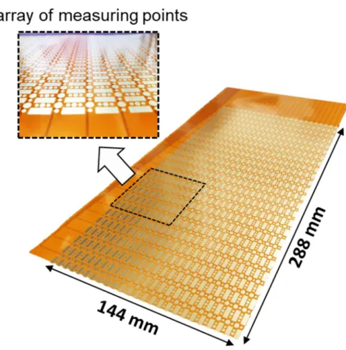
Figure 2.10 Fabricated sensor based on FPCB (24 × 24 array of measuring points) ... 32
Figure 2.11 Cross-sectional view of 4-layer FPCB ... 33
Figure 2.12 Circuitry system ... 33
Figure 2.13 Signal switching board ... 34
Figure 2.14 Change of measurement region by switching the signal ... 34
Figure 2.15 Layout of circuit composition ... 35
Figure 2.16 Calibration method ... 36
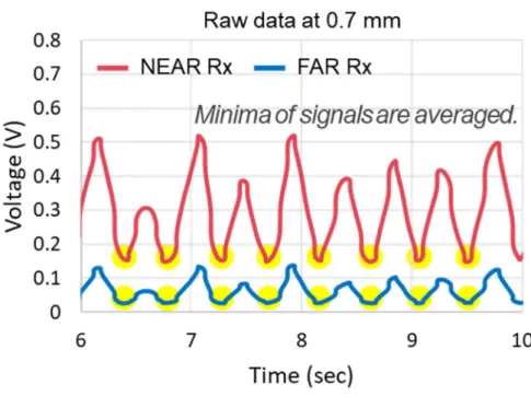
Figure 2.17 Raw data during sensor calibration at 0.7 mm liquid film ... 37
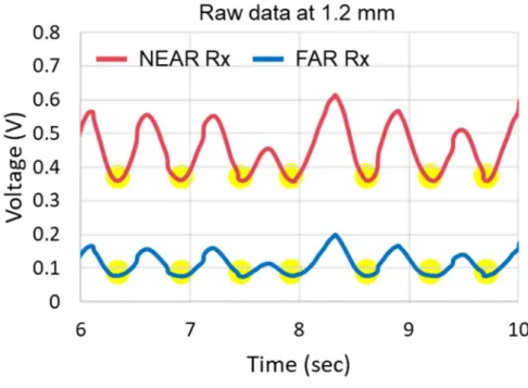
Figure 2.18 Raw data during sensor calibration at 1.2 mm liquid film ... 37
Figure 2.19 Calibration results ... 38
Figure 2.20 Determination of film thickness with two receivers ... 38
Figure 2.21 Advantage of current method for film thickness determination ... 39
Figure 3.1 Schematic of experiment facility ... 58
Figure 3.2 Schematic of test section ... 59
Figure 3.3 Photograph of test section ... 59
Figure 3.4 Photograph of liquid film with different water inlet velocities ... 60
Figure 3.5 Measurement of liquid film thickness with different water inlet velocities ... 60
vii
Figure 3.6 Measurement of liquid film thickness with different water inlet
velocities ... 61
Figure 3.7 Photograph of liquid film with different water inlet velocities (𝑗 , = 24 m/s) ... 62
Figure 3.8 Liquid film measurement with different water inlet velocities (𝑗 , = 24 m/s) ... 62
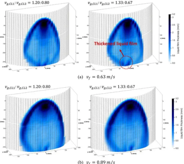
Figure 3.9 Liquid film measurement with different air velocities (𝑣 = 0.63 m/s) . 63 Figure 3.10 Change of the liquid film boundary with different air velocities (𝑣 = 0.89 𝑚/𝑠) ... 63
Figure 3.11 Liquid film thickness profile along the x-direction (𝑣 = 0.89 𝑚/𝑠) 64 Figure 3.12 Positions where liquid film off-take occurs... 64
Figure 3.13 Time-averaged liquid film thickness with different ratios of air inlet velocity (𝑗 , = 24 𝑚/𝑠) ... 65
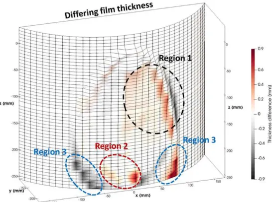
Figure 3.14 Difference between liquid film thickness at air velocity ratios of 1.33:0.67 and 1.00:1.00 (𝑣 = 0.63𝑚𝑠 and 𝑗 , = 24 𝑚/𝑠) ... 66
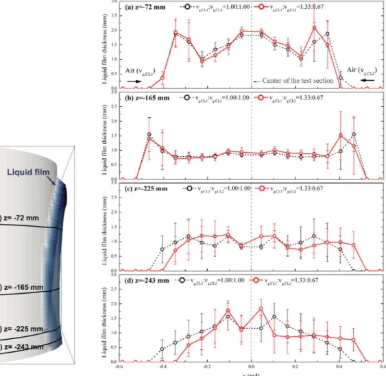
Figure 3.15 Liquid film thickness profiles with asymmetric air flow (𝑣 = 0.63𝑚𝑠 and 𝑗 , = 24 𝑚/𝑠) ... 67
Figure 3.16 Peak positions of liquid film boundary with 𝑣 = 0.63 𝑚/𝑠 and 𝑗 , = 24 𝑚/𝑠: (a) peak positions and (b) changes in peak positions with asymmetric airflow ... 68
Figure 3.17 Fluctuation of liquid film thickness with different air inlet velocities .... 68
Figure 3.18 Fluctuation of liquid film thickness with 𝑣 = 0.63 𝑚/𝑠 and 𝑗 , = 24 𝑚/𝑠: (a) fluctuation and (b) difference in fluctuation ... 69
Figure 3.19 ECC bypass fraction under symmetric airflow conditions ... 69
Figure 3.20 Shifted liquid film boundary with asymmetric air inlet flow ... 70
Figure 3.21 ECC bypass fraction under asymmetric airflow conditions ... 70
Figure 4.1 Relationship of diffusion velocity, slip velocity and mass-averaged velocity .. 89
Figure 4.2 Features of traditional two-phase flow models ... 89
Figure 4.3 Computational domain ... 90
Figure 4.4 Simulation for obtaining fully-developed flow as boundary condition 90 Figure 4.5 Meshing configuration ... 91
Figure 4.6 Transient simulation result (W089A00) ... 92
Figure 4.7 Spatio-temporal averaging film thickness in CFD ... 92
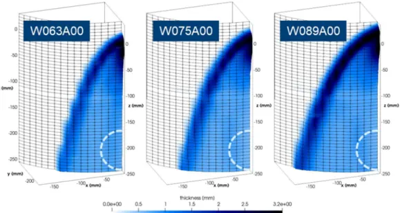
Figure 4.8 Comparison of liquid film distribution (W063A00, W089A00) ... 93
viii
Figure 4.9 Comparison of liquid film thickness (W063A00, W089A00) ... 93
Figure 4.10 Large discrepancies in film thickness near the film boundary (W089A00) 94 Figure 4.11 Determination of flow regimes using γ ... 94
Figure 4.12 Determination of using droplet diameter according to γ ... 95
Figure 4.13 Validity of film interface identification with γ ... 96
Figure 4.14 The computational cell where the droplet diameter is effectively used (cross-section of broken cold leg) ... 97
Figure 4.15 Bypass fraction according to the droplet diameter (W063A22) ... 97
Figure 4.16 Effect of B on spreading width of liquid film (W063A24) ... 98
Figure 4.17 Comparison of film spreading width (W063A24) ... 98
Figure 4.18 Bypass fraction according to B (W063A24) ... 99
Figure 4.19 Different film off-take phenomenon according to B ... 99
Figure 4.20 Determination of B for each simulation case ... 100
Figure 4.21 Comparison of bypass fraction in all simulation cases ... 100
Figure 4.22 Changes of bypass fraction with different B ... 101
Figure 4.23 Comparison of liquid film thickness (W063A20, B=10) ... 101
Figure 4.24 Comparison of liquid film thickness (W063A24, B=30) ... 102
Figure 4.25 Comparison of liquid film thickness (W063A28, B=30) ... 102
Figure 4.26 Determination of δ for each simulation case ... 103
Figure 5.1 Difficulties in simulating the film off-take with multiD component in safety analysis code ... 123
Figure 5.2 Liquid film off-take phenomenon governed by three parameters ... 124
Figure 5.3 Off-take volume divided into LEFT and RIGHT sections ... 124
Figure 5.4 CFD results extracted at junctions of off-take volume ... 125
Figure 5.5 Tracking of film boundary position at off-take volume ... 125
Figure 5.6 Prediction of film boundary position in the model ... 126
Figure 5.7 Comparison of predicted film boundary to the experiment results .... 126
Figure 5.8 Two factors affecting film off-take rate with respect to film boundary position ... 127
Figure 5.9 Two factors affecting film off-take rate ... 128
Figure 5.10 Distance between broken CL and film boundary ... 128
Figure 5.11 Normalized distance according to the air velocity ... 129
Figure 5.12 Normalized film offtake rate with 𝑊𝑒 . 𝑅𝑒 . ... 129
Figure 5.13 Normalized film offtake rate with 𝑊𝑒 . 𝑅𝑒 . 𝑅 ... 130
Figure 5.14 Normalized film offtake rate with 𝑊𝑒 . 𝑅𝑒 . 𝑅 𝐵𝑜 . ... 130
ix
Figure 5.15 Developed film model implemented as a film off-take model in
MARS source code ... 131
Figure 5.16 MARS multiD nodalization of SNU experiment ... 131
Figure 5.17 Simulation results of SNU experiment (Default MARS) ... 132
Figure 5.18 Simulation results of SNU experiment (Modified MARS) ... 132
Figure 5.19 Comparison of air velocity profile (W063A20) ... 133
Figure 5.20 Comparison of air velocity profile in all cases ... 133
Figure 5.21 Simulation results of SNU experiment (Modified MARS with adjusting loss coefficient) ... 134
Figure 5.22 Simulation results of SNU experiment under asymmetric airflow conditions (Modified MARS with adjusting loss coefficient) ... 134
Figure 5.23 Calculated bypass fraction at LEFT and RIGHT sections under asymmetric airflow conditions ... 135
Figure 5.24 Nodalization in DIVA simulation ... 136
Figure 5.25 Computational domain of DIVA simulation with CFD ... 137
Figure 5.26 Comparison of air velocity at cold leg side junction ... 137
Figure 5.27 Comparison of air velocity at hot leg side junction ... 138
Figure 5.28 Adjustment of loss coefficient ... 138
Figure 5.29 Calculated air velocity in MARS according to loss coefficient ... 139
Figure 5.30 DIVA validation result (KMA-DB 259-268) ... 139
Figure 5.31 DIVA validation result (KMA-DB 270-280) ... 140
Figure 5.32 DIVA validation result (KMA-DB 282-293) ... 140
Figure 5.33 Calculated bypass fraction at LEFT and RIGHT sections in DIVA simulation (KMA 282-293) ... 141
Figure 5.34 Effect of shifted DVI nozzle on the film off-take in each section .... 141
Figure 5.35 Comparison of bypass fraction in all SNU simulation cases ... 142
Figure 5.36 Comparison of bypass fraction in all DIVA simulation cases ... 142
Figure 5.37 MIDAS validation result ... 143
Figure 5.38 Different void heights in DIVA and MIDAS simulations ... 143
Figure 5.39 Little effect of void height on predicting air velocity in CFD simulation (DIVA KMA-273) ... 144
Figure 5.40 MIDAS simulation result with void height of 0.72 m ... 145
Figure 5.41 MIDAS simulation result without condensation effect ... 145
Figure 5.42 Experiment database for film spreading width with different geometrical configurations (Cho, 2004) ... 146
x
List of Tables
Table 2.1. Specification of CCS-PRIMA CL-4 ... 26
Table 3.1 Scaling ratio with the modified linear scaling methodology ... 56
Table 3.2. Accuracy of measurement instruments ... 56
Table 3.3. Test conditions ... 57
Table 4.1 Use of interface turbulence damping coefficient (B) with flow conditions ... 86
Table 4.2 Simulation conditions ... 87
Table 4.3 Droplet size measured in annular flow experiment ... 87
Table 4.4 Determination of B in SNU simulation... 88
Table 4.5 Determination of δ(m) in SNU simulation ... 88
Table 5.1 DIVA simulation cases ... 122
Table B.1 The source code to apply the developed film off-take model ... 167
1
Chapter 1 Introduction
1.1 Background and Motivation
1.1.1 Liquid film off-take in reactor vessel downcomer
In a nuclear power plant, various two-phase flow phenomena are expected to occur. In particular, in an accident condition, a liquid film can appear in the areas such as reactor core, reactor downcomer, and heat exchanger surface. The behavior of the liquid film is an important factor that impacts the safety analysis of a nuclear reactor and the evaluation of heat exchanger performance. Therefore, there have been many studies to investigate the thermal-hydraulic phenomena related to the liquid film. For example, condensation heat transfer through the liquid film has been studied to evaluate the performance of passive safety systems and the integrity of reactor cores and containments. Annular film dryout, which is one of the mechanisms of the critical heat flux (CHF) phenomenon, has been investigated because of safety concerns about the transients of pressurized water reactors (PWRs) and boiling water reactors (BWRs) with respect to their design and safety assessment. Moreover, an accurate description of the liquid film behavior in the reactor vessel (RV) downcomer has been attempted to determine the coolant flow
2
rate for core cooling and to provide experimental data for safety analysis code validation (MPR-1329, 1992, Kwon et al., 2003). As explained above, in a nuclear system, it is very important to investigate liquid film behavior accurately for safety assurance and design improvement.
The phenomenon of interest in the present study is the bypass of emergency core coolant (ECC) during the reflood phase of a loss of coolant accident (LOCA) in a PWR, as shown in Fig. 1.1. If a LOCA breaks out with a break in a primary coolant system of a PWR, the ECC is injected by the emergency core cooling system. The steam generated in the reactor core with the decay heat flows out through the broken cold leg, and some of the ECC bypasses out, off-taken by the steam flow. The bypassed ECC is then discharged from the break to the containment building. Depending on its temperature and pressure, it can evaporate in the nuclear reactor containment building, increasing the containment pressure or flow down, and accumulate in the containment sump. The more the ECC bypasses out, the less will be its contribution to the emergency core cooling. If the liquid flow is insufficient to remove the decay heat, the reheating of nuclear fuel rods may result.
For this reason, a number of experimental and analytical studies were carried out to better understand its mechanism and predict it more accurately (Bae et al., 2000, Cho et al., 2005, Yang et al., 2017). In the ECC bypass during the reflood phase, the key thermal-hydraulic phenomena are the interaction between falling liquid film, upward, or transverse gas flow, and droplet entrainment as those two determine the momentum transfer between two phases, and consequently, the fraction of the ECC bypass.
3
1.1.2 Challenges with multi-dimensional system code simulation
Under an accident condition in a light water reactor, a steam-water two-phase flow is established, and the interaction between each phase leads to complex thermal-hydraulic phenomena. With the increased need to predict more realistic flow behaviors, most of the nuclear reactor safety analysis codes have adopted multi-dimensional modules, for example, RELAP5-3D (Idaho National Laboratory, 2005), MARS (Korea Atomic Energy Research Institute, 2007), SPACE (Korea Hydro and Nuclear Power, 2012), TRACE (U.S. Nuclear Regulatory Commission, 2007), and CATHARE (Geffraye et al., 2011). They include the multi-dimensional modules for simulating multi-dimensional two-phase flows with increased accuracy.
The verification and validation (V&V) of the models and correlations in these codes have been carried out to improve the prediction capability of the modules. The MARS (Multi-dimensional Analysis of Reactor Safety) code has been developed by KAERI (Korea Atomic Energy Research Institute) for the multi-dimensional thermal-hydraulic system analysis of reactor transients (KAERI, 2007), and it is currently being used for the regulatory audit calculation by KINS (Korea Institute of Nuclear Safety) (Lee et al., 2016). It incorporates two different multi- dimensional modules; one is “Vessel,” which is dedicated to the reactor pressure vessel analysis, and the other is “MultiD,” which is used for general purpose applications. The former is based on the COBRA-TF code (Salko and Avramova, 2015) consolidated with the one-dimensional (1D) code, and the latter is newly developed by extending the one-dimensional code and adding the turbulent diffusion terms. In particular, the RV downcomer is the component in which the multi-dimensional flow appears as dominant under accident conditions. The phenomena that occur in the RV downcomer are of great importance for the reactor
4
safety analysis as they determine the behaviors of the emergency core coolant (ECC) and the safety systems.
However, even if the multiD module in the system code can consider multidimensional effects, it has inherent limitations in that the computational volume size cannot be configured to be as small as the CFD scale, and the momentum source terms in the two-fluid model are estimated using the 1D model dependent on flow regimes. Figure 1.2 shows a possible problem when the code interprets the liquid film off-take phenomenon in reactor downcomer. In a computational volume in which the film off-take occurs (off-take volume), the code does not recognize the actual liquid film configuration and assumes annular flow with a gas flow toward the broken cold leg. Then, the interfacial friction estimated for the annular flow regime causes liquid film to be off-taken to the broken cold leg;
this leads to an overestimation of the amount of water bypass.
To solve the issue described above, a film off-take model that correlates the branch quality and total gas flow rate for ECC bypass phenomenon was proposed and implemented in the system codes (KAERI, 2005). However, even if the existing film off-take model predicts the ECC bypass rate well under specific experimental conditions, it is still unclear whether it can cover a variety of flow conditions because the film off-take phenomenon may be more complicated than the way it is modelled with only the gas flow rate. This has motivated the development of a more physical film off-take model with identifying the major parameters other than air flow rate in this study. Here, to identify the parameters governing the film off-take phenomenon, there is need to investigate the local flow behaviors. Therefore, high- fidelity experiment and simulation studies were required in order to obtain local flow variables such as the liquid film thickness, liquid film velocity, and gas
5
velocity, which could provide a deeper understanding of film off-take mechanisms, enabling its use to model the local phenomenon.
1.2 Literature Review
1.2.1 ECC bypass experiment
In a previous experimental study for ECC bypass phenomenon, a direct vessel injection visualization and analysis (DIVA) test was carried out using air-water two- phase flow (KAERI, 2002). The DIVA test facility consists of the downcomer, four cold legs, two hot legs, air-water separator, four water injection systems, and a steam supply system. The four DVI nozzles are connected from the high-pressure safety injection (HPSI) simulators to the upper downcomer for injection of water.
There are three intact cold legs, which are the inlet of steam flow, and a broken cold leg, which functions as the exit of the air flow. The test sections were 1/7 and 1/5 APR1400 RV annulus downcomer, and they were made of transparent acryl to enable better visualization of the bypass phenomenon. From the visual observation, it was found that the flow regime in the downcomer is dominated by two- dimensional (2D) film flow during the late reflood phase of the LBLOCA (Cho, 2004). In addition, the ECC bypass fraction, which is defined as the ratio of the break water mass flow to the total injection water mass flow, was obtained in the test.
The multi-dimensional investigation in downcomer annulus simulation (MIDAS) test is a steam-water ECC bypass experiment in 1/5 APR1400 RV downcomer (Yun et al., 2002). The configuration of the test facility is similar to that
6
of DIVA. However, because the steam was used as the working fluid instead of air, a steam boiler was utilized to supply the steam flow. The maximum allowable operating conditions were a pressure of 10 bars and a temperature of 300℃. As in the DIVA test, the ECC bypass fraction was also measured in the MIDAS test.
In the experiment conducted by the Korea Advanced Institute of Science and Technology (KAIST), by using the test facility of plane-channel type scaled down to 1/7 ratio of the prototype reactor, the water film spreading width and ECC bypass fraction were investigated (Lee, 2004). Based on the results obtained from the water film spreading test, the curvature effect was found to be negligible.
The 1/10 air-water bypass tests were performed by Seoul National University (SNU) to assess and optimize the DVI system (KAERI, 2001). This study also focused on the ECC bypass measurement by considering the air-water flow characteristics in the scaled-down model. The results indicated flow characteristics that were similar to those of the DIVA test.
Another test conducted at SNU and KAERI was the 2D air-water film flow experiment (Yang et al., 2015). The experiment was performed in a 1/10 plane- channel type downcomer, and focused on the 2D behavior of liquid film without describing film off-take to the broken cold leg. Pitot tubes, a depth-averaged particle image velocimetry (PIV) method, and the ultrasonic gauge were applied to obtain the local measurement of the air velocity, the liquid film velocity, and the liquid film thickness, respectively. The measured data from the experiment were used to evaluate local wall and interfacial friction factors, and they were able to improve the predictability of the liquid film behavior with the nuclear safety analysis code MARS-KS.
As described above, most of the ECC bypass experiments focused on obtaining
7
the ECC bypass fraction rather than measuring local flow variables. Because of the insufficient local measurements of two-phase flow parameters under ECC bypass conditions, there have been limitations with respect to the CFD validation or improvement of the film off-take model. In the case of the air-water film flow experiment, even though local flow parameters such as the liquid film velocity and thickness were measured, the ECC bypass phenomenon was not described, and could not investigate the relationship between the local flow behavior and film off- take. Therefore, a new experiment was needed to provide local flow parameters under ECC bypass conditions in order to validate CFD simulation and to develop the film off-take model proposed in this study.
1.2.2 Liquid film thickness sensor
An appropriate measurement technique for flow parameters should be determined prior to setting up the high-fidelity experiment. To measure the liquid film thickness, Yang et al. (2015) used an ultrasonic gauge in the air-water film flow experiment. However, the ultrasonic gauge was found to be not an appropriate measurement method for applying to the high-fidelity experiment owing to the reasons given below.
First, the ultrasonic gauge is only available on the point measurement of the liquid film thickness. To obtain the field data at once, numerous sensors are required, which is not cost-effective. Furthermore, because of the physical size of the measurement sensor, installations with a high degree of integration are limited.
In addition to the ultrasonic method, techniques based on neutron, laser-induced fluorescence (LIF), electrical conductance and capacitance are capable of
8
measuring the liquid film thickness; each of them has strengths and weaknesses, as shown in Table 1.1. Among them, the electrical conductance method has been widely used to obtain a high temporal resolution because of its electrical characteristics and simple setup. In this method, the measuring point consists of a pair of electrodes, and the voltage drop between the two electrodes is used to obtain the liquid film thickness.
Recently, there have been studies that apply an array of multiple measuring points to the sensor and use it on a curved plane. Damsohn et al. (2010) fabricated an array of 64 × 16 measuring points on a flexible printed circuit board (FPCB).
FPCBs with substrates of polyimide film have great flexibility, so they are applicable to curved sections. This sensor was developed to measure the liquid film thickness in an annular flow that can be observed around BWR fuel rods. The size of a measuring point in the sensor is 2 mm × 2 mm for a maximum film thickness of 0.8 mm. To measure a thicker liquid film of up to 3.5 mm, Lee et al. (2017) enlarged the measuring point so that it consisted of ring-shaped electrodes with dimensions of 15 mm × 15 mm. The unique feature of this sensor is that it can be used in a temperature-varying condition by adopting the three-electrode method that uses the voltage ratio of two receiver electrodes. However, owing to the characteristics of electrical signals according to the distance between the transmitter and receiver, the measurement accuracy for very thin and thick film was confirmed to be low. This limitation that appears when measuring a wide range of film thickness values was also reported by Tiwari et al. (2014). In their study, a sensor was designed based on the same electrode shape from Damsohn et al. (2010). Then, the role of the electrode changed during the measurement to obtain three different measuring point sizes of 2 mm × 2 mm, 4 mm × 4 mm, and 12 mm × 12 mm for a
9
maximum film thickness of 3.5 mm. It was found that the measurable film thickness range was affected by the measuring point size because when the distance between the transmitter and receiver is short, the electrical signal is saturated in the thick film region, and when the distance is long, the electrical signal is saturated in thin film region.
Based on the results of this literature review, it was concluded that the electrical conductance method is an eligible measurement technique for covering a wide area of the liquid film and being applied to a curved surface, such as the downcomer annulus, and it was selected as the candidate measurement method for the present study. However, as noted above, the configuration of electrodes that constitute a measuring point should be carefully designed considering the target film thickness to prevent the measurement accuracy from decreasing.
1.2.3 CFD analysis
The field of CFD has come to occupy an important position in nuclear reactor safety analyses that require the accurate prediction of 3D geometrical effects for two-phase flow. Small-scale flow processes that are not seen by system codes can be accessed with CFD, which would result to in a better estimation of safety margins. Furthermore, in the case of this study, the local flow parameters such as liquid film velocity and gas velocity, which were not measured experimentally, could be obtained from CFD simulations, and could be used for modelling the film off-take phenomenon.
The prediction of the ECC bypass phenomenon using CFD codes was first attempted by Kwon et al. (2003). The objective of their study was to verify the
10
similarity of the velocity profile in the RV downcomer, which is scaled down based on the modified linear scaling method (Yun et al., 2004). A commercial CFD code, FLUENT ver. 5.5, is applied to analyze gas flow characteristics in a full-scale RV downcomer for the APR1400 and 1/5 scale for the MIDAS test facility. In addition, the spreading phenomenon of the ECC film on the inner downcomer wall was simulated using the volume of fluid (VOF) model, and it was validated based on experiment results.
Kwon et al. (2007) showed that CFD analysis could be extended to the two- phase film off-take phenomenon. Using the two-fluid model in CFX code, the DIVA test was simulated and the effect of the azimuthal angle of the DVI nozzle on the ECC bypass was quantified. As a result, the predicted ECC bypass fraction was in good agreement with the experimental data with the current DVI location (15°), but it was overestimated with the shifted DVI location (52°).
Yoon et al. (2015) numerically investigated the effects of the cross flow on the advanced DVI (DVI+) system for the new APR+ design. Then, the performance of the Emergency Core Barrel Duct (ECBD) was assessed by predicting the bypass fraction. To consider the two-phase flow of air and water, a homogenous model considering the surface tension and volume fraction at each phase was used. They quantitatively determined the fraction of the ECC water outside the ECBD by cross flow and derived the loss coefficient using the CFD analysis results.
As described above, in most of the previous CFD studies, the overall prediction capability of CFD codes for the two-phase phenomena was assessed by only comparing the calculation results of global parameters, such as the bypass fraction, with experimental data. This was because of the lack of local measurements of two- phase flow parameters, which did not enable the CFD code to be validated
11
sufficiently and which limited the model improvement. In the 2D air-water film flow experiment conducted by KAERI and SNU, although local liquid film velocity and thickness were measured, it was not possible to explain the ECC bypass using local flow behavior because the film off-take phenomenon was not described in the experiment.
In addition, the traditional two-phase flow models such as VOF and two-fluid model used in these studies are not very suitable for multi-regime flow, where continuous and dispersed phases coexist. This will be explained in detail in Chapter 4.
1.2.4 Modelling
In order to accurately predict the ECC bypass phenomenon with the system- scale codes, a thorough understanding of phase separation occurring near the branch is required. The liquid off-take and vapor pull-through for a branch connected to a horizontal pipe have been studied extensively with respect to SBLOCA, and the correlations had been built into RELAP/MOD3.3. However, the liquid off-take model in the branch connecting the vertical annular downcomer has not been provided in the existing system codes. Meanwhile, KAERI (2001) proposed a model that is applicable to the film off-take phenomenon in the downcomer based on DIVA and MIDAS test results. The form of the newly proposed film off-take model is the same as that of existing off-take model, and only the coefficients in the model are different. The model consists of critical height correlation (Smoglie, 1984) and branch quality correlation (Schrock et al., 1986), and it predicts the quality at the branch based on the gas flow rate. Even though this film off-take model became
12
available in the system codes, it could be concluded that the model was required to be further modified because the film off-take phenomenon may be more complicated than the way it is modelled with only the gas flow rate.
In the case of Yang et al. (2015), the correlations for wall and interfacial friction factors were developed based on the air-water film flow experiment. Then, they found that the developed wall friction model could yield a better estimation of the bypass fraction in the MIDAS simulation using the MARS multiD component.
Nevertheless, MARS overestimated the bypass rate under low gas flow conditions, which is an inherent limitation associated with the use of system codes. This means that a unique model, such as aforementioned off-take model proposed by KAERI, is required for the film off-take phenomenon, and is not simply described by the two-fluid model in the system codes.
All of the literature reviews including experiment, sensor, CFD analysis, and modelling are summarized and shown in Fig. 1.3.
1.3 Objectives and Scopes
The objective of this study is to model the film off-take phenomenon using local flow parameters obtained from high-fidelity experiments and CFD simulations. The contributions of this study are as follows: first, the liquid film thickness sensor was developed based on electrical conductance method. The developed sensor is an array-type, and is used to measure the field data and adopted the three-electrode method to widen the measurable film thickness range. Second, with the developed sensor, the local liquid film thickness and ECC bypass fraction were measured using an air-water film flow experiment (SNU experiment) that describes the film off-
13
take phenomenon. Third, the CFD analysis was performed with the VOF-slip model, and a parametric study was conducted to determine key parameters using simulations. Then, the simulation results were validated with the experimental data.
Fourth, the film off-take model was developed based on local flow parameters obtained from the CFD and experiment results. Finally, the developed film model validated with the results from the SNU experiment (1/10 scale) and DIVA test (1/5 scale) using the MARS multiD component. The outline of this study is described in Fig. 1.4.
14
Table 1.1 Comparison of measurement methods of the liquid film thickness Measurement
techniques Features
Neutron
- Neutron source
- Time-averaged measurement - High spatial resolution - Complicated setup
Ultrasound - Measurement of round-trip time of an ultrasonic wave
- Limitation in multiple-point measurements with high spatial integrity
Laser induced fluorescence (LIF)
- Measurement of emitted light of the fluorescent tracer using camera - High spatial resolution
- Limited temporal resolution with insufficient fluorescent light - Complicated setup
Conductance
- Measurement of electrical conductance of liquid film - High temporal resolution
- Simple setup
- Low spatial resolution
Capacitance - Measurement of electrical capacitance of liquid film - Measurement for non-conductive fluid
15
Figure 1.1 ECC bypass phenomenon
Figure 1.2 Limitation in current multi-dimensional code
16
Figure 1.3 Literature reviews
17
Figure 1.4 Outline of the study
18
Chapter 2
Liquid Film Thickness Sensor
In this chapter, the development process of the liquid film sensor is introduced.
The sensor is for efficiently obtaining local film thickness data, which can be used to validate the CFD analysis and to develop the physical model governing the film flow behavior. The contents included in this chapter have been published in Choi and Cho (2019).
2.1 Sensor Design
2.1.1 Features with flush-mounted electrode
The sensor designed in this study is based on the electrical conductance method, and it utilizes electrodes mounted flush to the substrate. A measuring point in the sensor consists of three different types of electrode: the transmitter electrode (Tx), receiver electrode (Rx), and ground electrode. The transmitter electrode transfers the electrical signal from outside the sensor to the receiver electrode, as shown in Fig. 2.1. In principle, the electrical potential difference between the transmitter electrode and the receiver electrode can be converted to the liquid film thickness, because the liquid film is related to the electrical resistivity covering both electrodes.
19
Here, the penetration depth which indicate the maximum film thickness the sensor can measure is limited by the distance between the transmitter electrode and the receiver electrode. In general, the penetration depth increases as the distance between two electrodes increases. However, in order to increase the spatial resolution of the sensor, the transmitter and receiver electrodes in each pair need to be placed as close to each other as possible. Besides, if the distance is far enough to measure the thick film (e.g., 3.5 mm), the sensitivity of signal according to the film thickness would be low in the very thin film region of less than 1 mm, which greatly reduce the measurement accuracy. This feature with flush-mounted electrode has been also confirmed in Tiwari et al. (2014). Therefore, in this study, it was necessary to design the electrode configuration in a new way to widen the measurable film thickness range.
2.1.2 Electrode design
In the present work, the size of a measuring point in the sensor was set to 6 mm
× 12 mm to measure the maximum film thickness of 3.2 mm, which was determined based on the results of a 2D film flow experiment using the slab-shaped test section (Yang et al., 2015). The configuration of the electrodes in the measuring point is proposed as illustrated in Fig. 2.2. This concept is based on that of Damsohn et al. (2010), but a special feature distinct from their design is that there are two different types of receiver electrode in a measuring area. These two electrodes, Rx- 1 and Rx-2, can be classified as the ‘‘NEAR Rx” and ‘‘FAR Rx,” according to their distance from the transmitter electrode. Obviously, the maximum film thickness that the sensor can measure is dependent on the relative location of the far receiver:
the longer the distance between the electrode and receiver, the thicker the
20
measurable film thickness. In the case of measuring a relatively thin film, however, the result based on the far receiver may have a large degree of uncertainty, because the relationship between the voltage drop and the liquid film thickness is nonlinear.
To compensate for this weakness, the NEAR Rx, was added in the measuring point.
Even if the near receiver is only available in a narrower range of film thickness compared with the FAR Rx, the sensitivity of the signal from it in the thin film region is better. Accordingly, by utilizing the results obtained from both receivers, measurement accuracy can be improved in a wider range of film thicknesses (Fig.
2.3).
Meanwhile, a cross-talk effect may exist, because the electrical current can be transferred from one transmitter to several receivers other than the receiver in the pair. In order not to degrade the measurement accuracy of the sensor, this effect needs to be reduced as much as possible, and for that purpose, ground electrodes were installed. The ground electrode was kept at a zero potential and served to reduce the cross-talk effect and to increase the penetration depth as well. In regard to the penetration depth, Damsohn et al. (2010) has reported that the further the ground reaches into the insulating gap between the transmitter and receiver electrodes, the higher is the penetration depth (Fig. 2.4).
In order to optimize the electrode configuration, COMSOL Multiphysics code (COMSOL, 2015) were used to analyze the electrical potential field with solving the Maxwell equation as below:
∯ 𝐸 ∙ 𝑑𝑆 = ∭ 𝜌𝑑𝑉 (2.1)
∇ ∙ 𝐸 = (2.2)
21
where 𝐸 is the electric field and 𝜖 is the permittivity of free space. Eqs. (2.1) and (2.2) are integral and differential equation respectively representing the gauss law of the electrical potential, which means that the electric flux out of enclosed surface is proportional to the total charge of the enclosed surface.
Figure 2.5 shows the computational domain in COMSOL analysis. Flush- mounted electrodes were covered with uniform liquid film with electric conductivity, and the other boundary of the bottom plane was set to insulated plane.
Electric potential of 5V was applied on the transmitter electrodes, and the ground potential was applied on the receiver and ground electrodes. Then, the developed electric field was shown in Fig. 2.6. The electric flux diffused from the transmitter and converged to the receivers and grounds.
During the optimization process we focused on to increase the signal sensitivity according to the liquid film thickness and to minimize the cross-talk effect. As shown in Figs. 2.7 and 2.8, electric field analysis was performed by changing the electrode size and shape, and the final determined shape was presented in Fig. 2.9.
Based on the final configuration, a measurement point was extended to an array of 24 × 24 measuring points, and it was fabricated on an FPCB to obtain the distribution of film thickness (Fig. 2.10). The copper electrode was covered by a nickel layer, followed by a thin protective layer of gold. The circuit wires in the FPCB were arranged in four different layers according to the type of electrode connected to them. Figure 2.11 shows a simplified cross-sectional view of the fabricated sensor.
22
2.1.3 Circuitry design
In order to acquire the data from the three electrodes (Tx, Rx-1, Rx-2), three signal lines for each probe are required in general signal processing methods. In the case of multiple-point measurement system such as N × N array, 3N signal lines are needed and this amount of signal lines require massive DAQ (Data Acquisition) devices.
Wire-mesh circuity system has the circuit pattern, which can address the above problem with crossing the signal lines of transmitters and receivers (Damsohn et al., 2010). The transmitter electrodes located in the same row are connected in parallel, and the receiver electrodes located in the column are coupled in parallel. The inducing signal is supplied to the first transmitter line and measurement is conducted in the sensors which are connected to the first transmitter line. After measuring and recording are finished, the inducing signal is switched to next transmitter line. As a result, the data from entire measurement points can be obtained by successive signal switching, which can reduce the number of signal lines to 2N for N × N array sensor system.
In this study, the circuitry system is modified to apply on the three-electrode method as illustrated in Fig. 2.12. For the N × N array sensor system, N signal lines are deposed for transmitters and 2N signal lines are deposed for receivers.
The signal lines of transmitters and receivers are crossed with similar pattern of the wire-mesh circuitry. Voltage signal (AC sine wave) is induced to transmitter line and 2N of receiver lines transfer the currents, and the measurement for liquid film thickness is proceeded successively with changing the connecting nodes by the use of the switching board (Fig.2.13). Figure 2.14 shows the change of active measurement region by switching the induced signal to the transmitter lines. When
23
a signal is applied to the first channel, the measurement region connected to induced transmitter line becomes active. By switching the induced signal, when it is applied to the second channel, then the active measurement region changes as shown in the figure. The layout of circuit composition in the sensor is shown in Fig. 2.15.
2.2 Sensor Calibration
2.2.1 Calibration method
For the sensor calibration, the method proposed by Ito et al (2016) was utilized.
The calibration method is illustrated in Fig. 2.16. This figure shows the liquid film sensors attached to the acrylic curved plate and the calibration plate beneath the sensors. The diameter of the curved plate was 400 mm, which was 1/10.93 of the inner diameter of the Advanced Power Reactor 1400 (APR1400) RV downcomer.
To minimize the measurement error caused by the curvature effect, the sensor was calibrated while attached to the curved plate. A calibration plate was installed to generate a certain film thickness, and the inner part of it was dented to a target calibration thickness. Total six calibration plates were used to form different liquid film thicknesses (0.2 mm, 0.7 mm, 1.2 mm, 2.2 mm, 2.7 mm, and 3.2 mm). The error of the gaps in the calibration plates was quantified using a confocal chromatic sensor (CCS-PRIMA CL4), and it was included in the uncertainty analysis. The specification of the CCS was presented in Table 2.1.
When the curved plate is on the calibration plate and sunk under water, a uniform liquid film is formed in the gap between the calibration plate and the sensor.
Afterward, the curved plate is rolled back and forth; then, the gap size of the calibration plate becomes the minimum film thickness that each measuring point
24
can have. The local minima of the signal were obtained when rolling the curved plate, and the values were used for the calibration as the voltage drop values that corresponded to the thickness of the dent (Figs. 2.17 and 2.18). The temperature and conductivity of the water used in the calibration were 20 ℃ and 6 𝜇𝑆/𝑐𝑚, respectively, and the same values were maintained during the experiment.
2.2.2 Calibration result
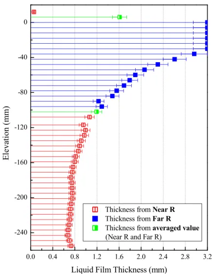
The calibration results at a measuring point in the film thickness range of 0.2 mm to 3.2 mm are presented in Fig. 2.19. In this graph, the normalized voltage means the measured voltage divided by the voltage at the film thickness of 3.2 mm.
The error bars indicate the uncertainty of the calibration plate assessed by the CCS sensor and the two-sigma range of the measured voltage. The two calibration curves obtained from the FAR Rx and NEAR Rx have different characteristics from each other. In the case of the NEAR Rx, the sensitivity of the signal according to the film thickness is high in the thin-film region (approximately 0.2–1.2 mm), but the signal increment becomes nearly saturated at 2.8 mm. On the other hand, in the case of the FAR Rx, steeper inclination of the signal is confirmed in the thick-film region (approximately 1.2–3.2 mm), although its sensitivity is low in the thin-film region.
Based on these results, the method for determining the film thickness is proposed that a set of calibration results from two receivers is selectively used considering the reference film thickness of 1.2 mm (Fig. 2.20). This has the advantage of improving the measurement accuracy of the sensor for wide range of film thickness.
The accuracy of the sensor can be defined as the uncertainty in the calibration process. Considering the two-sigma value of the measured voltage and the unevenness of the calibration plates, the maximum error of the calibrated sensor
25
was estimated to be 8%.
Meanwhile, our previous work confirmed that the calibration result worked successfully when it is applied to the liquid film with gas-liquid interface; the comparison showed good agreement between the result from the developed film sensor and the ultrasonic thickness gauge. Figure 2.21 shows the advantage of current method for film thickness determination. In thick film region, accuracy of the NEAR Rx measurement is relatively low, which shows large discrepancy in film thickness measurement. On the other hand, in thin film region, accuracy of the FAR Rx measurement is relatively low, which shows large discrepancy in film thickness measurement.
26
Table 2.1. Specification of CCS-PRIMA CL-4 Specification
Measuring range 4000 𝜇𝑚
Working distance 16.5 mm
Static noise 110 nm
Max. linearity error 300 nm
Min. measurable thickness 110 𝜇𝑚
27
Figure 2.1 Working principle of electrical conductance method
Figure 2.2 Electrode design
28
Figure 2.3 Adoption of two receivers (NEAR Rx and FAR Rx)
Figure 2.4 Sensor characteristic for different ground electrode shapes (Damsohn et al., 2010)
29
Figure 2.5 Computational domain in COMSOL
Figure 2.6 Electrical potential analysis using COMSOL
30
Figure 2.7 Design optimization with changing size of receiver electrodes
Figure 2.8 Design optimization with changing shape of ground electrodes
31
Figure 2.9 Final configuration of electrodes
32
Figure 2.10 Fabricated sensor based on FPCB (24 × 24 array of measuring points)
33
Figure 2.11 Cross-sectional view of 4-layer FPCB
Figure 2.12 Circuitry system
34
Figure 2.13 Signal switching board
Figure 2.14 Change of measurement region by switching the signal
35
Figure 2.15 Layout of circuit composition
36
Figure 2.16 Calibration method
37
Figure 2.17 Raw data during sensor calibration at 0.7 mm liquid film
Figure 2.18 Raw data during sensor calibration at 1.2 mm liquid film
38
Figure 2.19 Calibration results
Figure 2.20 Determination of film thickness with two receivers
0.0 0.2 0.4 0.6 0.8 1.0
0.0 0.4 0.8 1.2 1.6 2.0 2.4 2.8 3.2
0.0 0.2 0.4 0.6 0.8 1.0
0.0 0.4 0.8 1.2 1.6 2.0 2.4 2.8 3.2
0.0 0.2 0.4 0.6 0.8 1.0
0.0 0.4 0.8 1.2 1.6 2.0 2.4 2.8 3.2
Liquid film thickness (mm)
Normalized voltage (FAR Rx) NEAR Rx
FAR Rx
Normalized voltage (FAR Rx) Normalized voltage (FAR Rx)
39
Figure 2.21 Advantage of current method for film thickness determination
40
Chapter 3
Experiment for Two-phase Film Flow
An experimental work was carried out to investigate the film off-take under ECC bypass conditions using the developed film sensor. This chapter comprises the scaling method, experimental setup, and experimental results, which have been have been published in Choi and Cho (2019, 2020).
3.1 Scaling for ECC bypass phenomenon
To derive the important dimensionless parameters of the ECC bypass phenomenon, film flow analysis associated with gas-liquid the cross-flow was performed by Cho et al. (2005). In this analysis, the Wallis parameter has been derived as a dominant dimensionless parameter, which starts from the momentum equation for a control volume. The Wallis parameter was originally derived from the counter-current flow limitation (CCFL) analysis by Wallis (1969), but also has been widely accepted as one of the dominant dimensionless numbers regarding ECC bypass. In the present work, the original Wallis number was extended to the two-dimensional control volume considering flow direction in the downcomer of the direct vessel injection. The definition of the Wallis parameter is as follows.
41
𝑗∗ = 𝛼𝑣
/
= ̇
/
(3.1)
where 𝛼, 𝑣 , 𝑚̇ , 𝜌 , 𝐷 , and 𝐴 denote the volume fraction, the velocity of k-phase, the mass flow rate of k-phase, the density of k-phase, the downcomer gap size, and the flow area, respectively. The Wallis parameter is expressed as the ratio of the inertia force and gravitational force, and it works as a dominant parameter when the balance between the interfacial friction and gravitational force is important. This dimensionless number is often referred to as the modified Froude number or densiometric Froude number.
The modified scaling method (Yun et al., 2004), which was developed based on the Wallis parameter, was applied in the present experiment. In this scaling method, the velocity ratio was reduced to the square root of the length ratio to preserve the Wallis parameter between the prototype and the model. Scaling ratios for major parameters including the velocity, void fraction, and time were shown in Table 3.1 when the modified scaling method is applied. It preserves the aspect ratio of the geometry, as the conventional linear scaling method does, but requires reduced time and velocity compared with the prototypic. This requirement is expected to preserve the balance between the interfacial friction and gravitation forces.
The details of the validation of the scaling analysis are explained in Cho et al.
(2005). In the study, the experimental data produced in the 1/1, 1/4.0, 1/7.3 scale tests were compared with each other. The validation results showed that the liquid film spreading width and the ECC bypass fraction were well preserved with the scaling method. Although the effect of the interfacial heat transfer between the steam and ECC water was not considered in the derivation of the modified scaling method, it is still valid to investigate the dynamic interaction between two phases
42
in the ECC bypass condition.
Meanwhile, an ECC bypass experiment conducted in a full-scale downcomer geometry, UPTF-Test 21D, found that the condensation efficiency was close to the unity during the reflood phase of LBLOCA (MPR-1329, 1992), which means that the liquid film temperature increased up to the saturation temperature. If the liquid becomes saturated, no more condensation occurs and the two-phase flow becomes isothermal. This experimental result supports that the application of the modified linear scaling is an appropriate approach to preserve the ECC behavior in the reduced scale test facility using air and water as the working fluids.
3.2 Experimental Setup and Conditions
3.2.1 Experiment facility
To experimentally investigate the film off-take phenomenon under ECC bypass conditions, the air-water experiment facility was designed. A schematic diagram of the test facility is presented in Fig. 3.1. The major systems of the facility comprise an air injection section, water injection section, and air–water separation section. In the air injection section, the air is supplied into the test section through two pipes corresponding to the intact cold legs using the two air blowers. The angles between the two intact cold legs and the center of the test section were -60° and +60°. The test section describes the RV downcomer, and the shape of it is half of the downcomer annulus. To visualize the film flow in the test section, it was made of transparent acryl. The inner wall of the annular test section can be separated into three parts, and the middle part was corresponding to the curved plate utilized in
43
the sensor calibration. The film sensor attached on the curved plate measures the film thickness in the region between the DVI nozzle and the cold legs. The test section is a 1/10 scale model of the APR1400. In the actual plant, the angle between the ECC injection nozzle and the broken cold leg is 15°, but the nozzle in the facility is placed at the same angle with the broken cold leg, which has advantageous of these fundamental investigations and modelling the test section with the nuclear reactor safety analysis codes. A schematic and the actual shape of the test section are shown in Figs. 3.2 and 3.3, respectively. A valve to control the water level was connected to the lower part of the test section. Because of the constant water level in the test section, the injected air could not pass through the bottom of the test section, and the air–water separator became the only exit for the air. The pipe connecting the test section and the separator represented the broken cold leg. In the air–water separation section, a two-phase mixture from the test section was separated into water and air by the gravitational force through a perforated plate.
The air was discharged through the top of the separator, and the water was returned to the water tank.
In the air injection section, a thermal mass flow meter was installed in each cold leg to measure the air inlet velocity. Two electromagnetic flow meters were used to measure the water inlet velocity and the water penetration velocity. The temperatures in the air and water injection sections were measured by K-type thermocouples. All details of the instruments used are presented in Table 3.2.
3.2.2 Test matrix
The boundary conditions in the test were determined based on the transient
44
analysis results of the APR1400 during a cold leg break LOCA (KAERI, 2002).
According to the modified linear scaling method, the water velocity was varied in the range of 0.63 to 0.89 m/s, and the air velocity was varied in the range of 0 to 14 m/s for each intact cold leg. In an actual RV of APR1400, three intact cold legs are arranged asymmetrically with respect to the broken cold leg. Therefore, the gas does not flow symmetrically to the broken cold leg under actual conditions. Because the simplified test section with two intact cold legs and a broken cold leg was used in the test, the air inlet velocities at the two inlets had to be different to generate an asymmetric airflow distribution around the broken cold leg. Therefore, the ratio of the air inlet velocity (𝑣 , :𝑣 , ) was changed from 1.00:1.00 to 1.33:0.67, based on the real arrangement of the three intact legs, maintaining a constant air outlet velocity. Table 3.3 gives the test conditions including the water inlet velocity, 𝑣 , and air superficial velocity at the outlet, 𝑗 , , which are also provided with the Wallis parameter and Reynolds number. To calculate the Wallis parameter defined by the Eq. (3. 1), the mass flow rate at the inlet boundary was obtained instead of the void fraction which was unknown locally. In the case of calculating 𝑗∗, the total gas mass flow at the outlet was used for 𝑚̇ , and the vertical cross-section of the downcomer (annulus gap × diameter of cold leg) was used for 𝐴 . In the case of calculating 𝑗∗ , the horizontal cross-section of the downcomer was used for 𝐴 (annulus gap × arc length of annulus). The Reynolds numbers for liquid and gas phases were estimated with the inlet and outlet boundary conditions, respectively. The water conditions used in the experiment were the same as those used in the sensor calibration.
The uncertainties of the measured values in the test were analyzed for major measurement parameters. Based on the error propagation theory, the uncertainty of
45
the water mass flow rate was calculated with the uncertainties of the volumetric flow rate and the water density that is related to the temperature. These uncertainties of the measurement parameters were estimated by considering the instrument accuracy as a bias error and the deviation in the measurement as a precision error.
Then, the uncertainty of the bypass fraction was obtained with the uncertainties of the water inlet mass flow rate and the water penetration mass flow rate. The details of the uncertainty of the bypass fraction are given in Appendix A. For the uncertainty of the liquid film thickness, the bias error that was confirmed to be 8%
in the sensor calibration and the precision error were considered. In the experiment, the liquid film is fluctuating by the interaction with gas and its nature. Thus, the measurement data showed significant oscillation where the thick liquid film existed.
This fluctuation was regarded as the precision error of the thickness measurement, which was used for the uncertainty analysis.
3.3 Experimental Results
3.3.1 Time-averaged film thickness
Symmetric airflow conditions
Under the symmetric airflow conditions, the distribution of the liquid film thickness was measured using the developed sensor. The data acquisition continued for 10 sec for one transmitter line with the time resolution of 0.04 sec so that 250 samples of the raw data were acquired. Then, the time-averaged film thicknesses could be obtained. Next, the activated transmitter line was switched using the signal switching board, and the procedure was repeated until the whole measurement area