Estimation of the Reference Evapotranspiration using Daily Sunshine Hour

Estimation of the Reference Evapotranspiration using Daily Sunshine Hour

Khil-Ha Lee* Hongyeon Cho**

Civil Engineering, Daegu University*

Marine Environment and Conservation Research Department, Korea Ocean R&D Institute**

(Manuscript received 17 February 2011; accepted 24 August 2011)

일조시간을 이용한 기준 증발산량 추정

이길하*·조홍연**

대구대학교 토목공학과*, 한국해양연구원 해양환경보전연구부**

(2011년 2월 17일 접수, 2011년 8월 24일 승인)

Abstract

이 논문에서는 일사량과 일조시간에 관한 통상적인 선형관계식보다 정확한 비선형 관계식에 대한 적용검토를 수행한다. 일조시간을 이용한 일사량 추정에 이어서 Penman-Monteith 방정식을 이 용하여 기준 증발산량을 추정하였다. 우리나라 20개 지점의 1997년부터 2006년까지의 일사량 및 일조시간 자료를 포함한 기상자료를 이용하여 선형 그리고 수정 비선형 Angstrom 방정식을 보정 하고 기준 증발산량을 추정하였다. 일조시간과 일사량 사이의 선형과 비선형 관계식을 이용한 기준 증발산량의 상대비교를 수행하였다. 선형 및 비선형 관계식을 이용한 방법 모두 RMS 오차는 5.96, NSC(Nash-Sutcliffe Coefficient)는 0.95로 추정되었고, 그 차이는 매우 미미하였다. 그러나 상 대적으로 일사량이 기준 증발산량에 크게 기여하는 하계에는 그 차이가 증가하기 때문에 보다 개선 된 비선형 관계식을 이용하는 방법에 대한 엄밀한 검토가 필요하다.

주요어 : Modified Angstrom equation, Reference evapotranspiration, Solar radiation, Bright sunshine duration, Penman-Monteith equation

Corresponding Author: Hongyeon Cho, Marine Environment and Conservation Research Department, Korea Ocean R&D Institute, Ansan PO Box 29, Seoul 425-600, Korea Tel:+82-31-400-6318 Fax:+82-31-400-7868 E-mail : [email protected] 연구논문

I. INTRODUCTION

In places where solar radiation (R_S) is not mea- sured directly, it can be estimated by interpola- tion from nearby localities where radiation data are available, by using models and empirical cor- relations, starting with the more diffusely known meteorological data or by using a combination of methods (Allen,1995; Allen, 1997; Lee, 2009a). A typical example of the second method is the cor- relation found by Angstrom (1924) and others between global solar radiation (R_S) and bright sunshine duration (hours, n) and measured at many meteorological stations. This relationship to draw solar radiation estimates is used more often than those estimates determined by using only direct measured radiation data.

The Angstrom equation (Angstrom, 1924;

Prescott, 1940) has long been a dominant tool to use as a basis approach to estimate the R_S. The Angstrom equation is a very convenient tool for a large number of locations (Annear and Wells, 2007; Gopinathan, 1988); however, many scien- tists have presented slightly different model para- meters for different locations (Doorenbos and Pruitt, 1977). Atmospheric constituents, such as molecules, aerosols, and clouds, can affect solar radiation, and these atmospheric constituents should be included in building the relationship between R_S and bright sunshine hours (n).

Consequently other attempts have been made to modify the Angstrom equation, including the use of more meteorological parameters, such as sur- face albedo, latitude, ambient temperature, total precipitation, humidity, elevation, amount of cloud cover, etc. (Dorvlo and Ampratwum, 2000;

Hargreaves et al., 1985; Hay, 1979; Supit and van Kappel, 1988). However, the additional meteoro- logical parameters needed to improve the origi-

nal Angstrom equation could present a bottle- neck for these previous approaches. Hence, Lee (2009b) recently suggested a simple nonlinear form of the modified Angstrom equation to improve both its accuracy and fitness. It showed successful performance. This study focused on the simple modified Angstrom equation.

Evapotranspiration (ET) as a major component of the hydrologic cycle will affect crop water requirement and future planning and manage- ment of water resources. Estimates of reference evapotranspiration (hereafter ET₀) are an impor- tant input to hydrologic models and the present models generally do not provide direct estimates of ET₀from the land surface. Management of regional and local water resources and irrigation has required the use of an empirical equation to estimate ET₀. Either a relatively accurate equation or a simple equation usually requires solar radia- tion data as an essential input variable; yet in most cases the available network of meteorologi- cal stations does not allow direct measurement or even an estimation of incoming solar radiation.

In this study, the modified Angstrom equation was facilitated at 20 meteorological stations on the Korean Peninsula. Then ET₀was calculated and tested against reference values to see how the modified Angstrom equation affects ET₀. This study is meaningful in the sense that temperature and solar radiation can explain at least 80% of ET₀ (Vanderlinden et al., 2004; Samani, 2000;

Priestly and Taylor, 1972). The results show that both the original and the modified equation pre- sent a similar level of performance once they are locally calibrated, and the modified Angstrom equation is not able to provide superiority in terms of accuracy.

II. METEOROLOGICAL DATA

The meteorological data used for the study were provided by the Korea Meteorological Administration (KMA), corresponding to the period of 1997-2006 (total 120 months) and con- sisting of 3,652 carefully screened daily values.

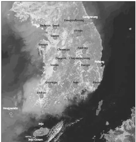
All the stations were close to the reference condi- tion (Allen, 1996). A summary of site informa- tion, including daily manual observations, such as mean temperature, relative humidity, wind speed, and solar radiation (R_S) at the 20 stations (12 inland and 8 coastal, including island:

Stations 16 and 17) appear in Table 1 (see Fig. 1).

Study sites were selected on the basis of data completeness and reliability. Those days when

observations were not available were averaged and filled with neighboring values. The mea- sured weather data was checked for integrity, quality, and reasonableness. Data quality and integrity checks were made and followed up on, using precedent-setting studies (Irmak et al., 2003a; Temegsen et al., 1999; Allen, 1996) for all locations. In the temperature data quality check, the measured maximum and minimum air tem- perature (T_max and T_min, respectively) data for each individual year were compared against the long- term temperature extremes. The deviation of dew point temperature (T_dew) from T_min was within 3-4 ˚C for the substantial portion of the records for all locations. To check the integrity of Rs, clear sky envelopes (Allen, 1995; Allen, 1997)

Figure 1. Study region and meteorological stations(The base map is the GOCI image provided by the Korea Ocean Satellite Center, KORDI)

were calculated. There was some mismatch between the measured and the clear sky radia- tion envelope because some points never reached a clear sky. These points needed further scrutiny;

adjustment multipliers were applied to force the upper surface of measured R_Sto reach computed clear-sky radiation envelopes. This adjustment was based on the assumption that there are com- monly some clear-sky days at each location and that a single factor could produce suitable cali- bration correction for the measurement (Allen, 1996).

Solar radiation is measured using pyranome- ters of the CMP21 and sunshine duration with the MS-093. Expected daily accuracy of the pyra-

nometers is 2%, and the integration error of the sunshine duration meters is less than 10min/day.

The data used for the study were daily averages on a horizontal surface. Table 1 also presents a summary of weather stations, including geo- graphical coordinates, elevation, and measure- ment height. Stations 6 and 12 were located in a mountainous area and influenced by the oro- graphic effect. The logarithm wind profile equa- tion (Brustaert, 1991) was used to adjust the mea- sured wind speed at each height to a reference height of 2m. The Korean Peninsula has a mod- erate climate that is characterized by distinct wet and dry seasons. The dry season coincides with the Northwest wind, which is predominant from Table 1. Summary of weather stations used for the study. Ele. = elevation (m), Lat. = latitude (degree), Lon. = longitude(degree), H_t = height of thermometer above the ground(m), H_w = height of anemometer above the ground(m), R_s = Incoming Solar Radiation (MJm^_2d^_1), Sunhr=bright sunshine duration(hours), WS = wind speed(m/sec), RH = relative humidity(%), Tmean = daily mean temperature(˚C). The mean and standard deviation values for all variables are for the period of the study (1997-2006).

Station Station Ele. Lat. Lon. H_t H_w Mean Std

index. name Rs Sunhr WS RH T Rs Sunhr WS RH T

1 Andong 140.7 36.57 128.70 1.5 15.5 13.65 5.90 1.57 65.44 12.42 6.12 3.69 0.82 15.48 9.74 2 Cheongju 56.4 36.63 127.43 1.5 10.0 13.10 5.86 1.81 64.71 13.25 8.53 3.78 0.90 13.26 10.02 3 Chupungnyeong 242.2 36.22 127.98 1.5 20.7 12.67 5.85 2.53 66.06 12.27 6.58 3.89 1.60 15.06 9.56 4 Deagu 57.4 35.88 128.62 1.5 18.2 13.08 6.10 2.37 59.14 14.83 6.31 3.82 1.00 16.04 9.26 5 Daejeon 62.6 36.37 127.37 1.6 22.8 13.48 5.86 1.92 67.22 13.47 6.71 3.73 1.03 14.02 9.78 Inland 6 Daegwallyeong 790.0 37.67 128.72 1.8 10.0 12.73 5.79 4.29 74.22 7.39 7.10 4.05 2.53 17.33 9.84 7 Gwangju 74.5 35.17 126.88 1.5 17.5 13.65 5.56 2.09 67.15 14.53 6.69 3.65 0.95 13.00 9.23 8 Jeonju 61.1 35.82 127.15 1.5 18.4 12.82 5.50 1.79 68.04 14.24 6.34 3.71 0.76 12.55 9.67 9 Jinju 27.1 35.15 128.03 1.5 10.0 13.65 6.09 1.61 67.67 13.99 6.52 3.76 0.88 14.59 9.34 10 Seoul 85.5 37.57 126.95 1.5 10.0 11.68 5.10 2.17 62.64 13.27 6.37 3.59 0.88 14.24 10.18 11 Suwon 34.5 37.27 126.98 1.5 20.0 13.31 5.80 1.89 65.33 12.83 6.55 3.79 0.86 13.81 10.23 12 Wonju 150.7 37.33 127.93 1.6 10.0 12.88 5.32 1.08 67.94 12.26 6.57 3.59 0.64 13.28 10.48 13 Busan 69.2 35.10 129.02 1.7 17.8 13.27 6.08 3.47 63.73 15.41 6.70 3.84 1.36 18.84 7.97 14 Gangneung 26.1 37.75 128.88 1.7 13.8 12.81 5.82 2.81 59.11 13.71 6.61 3.94 1.26 20.51 8.98 15 Incheon 54.6 37.47 126.62 1.4 11.0 13.30 6.15 2.47 67.65 13.24 7.36 3.83 1.26 14.11 9.75 Coast 16 Jeju 19.9 33.50 126.52 1.8 12.3 12.81 5.06 3.23 68.16 16.37 7.70 4.11 1.48 12.42 7.59 17 Jejugosan 70.9 33.28 126.15 1.8 10.0 13.14 5.40 7.42 74.39 15.87 7.81 4.12 4.13 12.85 7.27 18 Mokpo 37.4 34.82 122.37 1.5 15.5 14.08 5.92 3.82 71.20 14.45 7.08 3.91 1.98 12.09 8.85 19 Pohang 1.3 36.02 129.37 1.6 13.2 13.27 6.12 2.72 61.85 14.95 6.64 3.97 0.92 18.95 8.69 20 Seosan 25.2 36.77 126.48 1.4 20.2 13.40 5.81 2.60 72.71 12.39 6.67 3.84 1.35 10.48 9.87

Station Station Ele. Lat. Lon. H_t H_w Mean Std

index. name Rs Sunhr WS RH T Rs Sunhr WS RH T

November to March. The wet season results from the Southeast wind, which brings moisture-laden air from the Pacific Ocean. That season lasts from May to October and accounts for 70 % of the annual precipitation. July-August is usually the wettest season. All sites exhibit typical daily and seasonal variations in moderate temperature trends, ranging between a seasonal maximum from April to October to a minimum from November to March. Coastal sites show less vari- ability in temperature, with a diurnal tempera- ture range (DTR) of approximately 7 ˚C.

The net radiation was computed using the measured shortwave R_S and the outgoing long- wave radiation equation (Irmak et al., 2003c) as follows;

Rn = R_ns_ R_nl (1)

in which, Rn=net radiation (MJ/m²/day);

R_ns=the rate of incoming net shortwave radiation (MJ/m²/day); R_nl = the rate of outgoing net longwave radiation (MJ/m²/day).

The incoming net shortwave radiation was cal- culated as follows;

R_ns= Rs(measured) (1-a) (2)

in which, a = surface albedo and 0.23 was used for grass reference crop surface; Rs(measure)

=total incoming (measured) solar radiation (MJ/m²/day).

The rate of outgoing net longwave radiation was expressed quantitatively as

R_nl= s

[ ]

III. THEORETICAL BACKGROUND

1. The Angstrom Equation

Angstrom (1924) and Prescott (1940) suggested a correlation in linear form as follows;

= a + b

( )

( )

where R_sis the total incoming shortwave solar radiation (MJ/m²/day); R_ais the extraterrestrial radiation (MJ/m²/day); a and b are the model parameters; n is the bright sunshine duration (hour); and N is the total day length (hour). To compute the extraterrestrial radiation R_aand total day length N, the following equations are used.

R_a= 15.392d_r(w_ssin f sin d + cos j cos d sin w_s) (5)

N = w_s (6)

d_r= 1 + 0.033 cos(2pJ/365) (7)

w_s= arccos(_ tan f tan d) (8)

d = 0.4093 sin(2pJ/365 _ 1.405) (9)

where Ra = extraterrestrial radiation (equiva- lent evaporation [mm/day] = 0.408 Radiation [MJ/m²/day]); d_r= relative earth-sun distance (-);

w_s = sunset hour angle (radians); j= latitude of site (+ for northern hemisphere, - for southern hemisphere) (radians); d= solar declination (radi- ans), and J = Julian days.

In equation (4), n/N denotes the cloudiness fraction, while Rs/Ra is affected by various atmospheric conditions, as stated earlier.

The input of extraterrestrial shortwave radia- tion Ra is absorbed by atmospheric gases, partic- ularly water vapor and ozone, and is scattered by air molecules and aerosol particles in clear sky conditions and additionally by clouds when these clouds are present (Maidment, 1993). Equation (4) is generalized in an attempt to improve accuracy and performance as follows and so called the

24 p

n N n

N R_s R_a

R_s R_so T⁴_max+ T⁴_min

2

“modified Angstrom equation” (Lee, 2009b);

= a + b

( )

( )

An additional parameter c, which describes the influence of the impeding factor and nonlinearity between Rs/Ra and n/N, is introduced in the equation (10). The original Angstrom equation (4) is a special form of the modified angstrom equa- tion (10), giving c=1.0 (Lee, 2009b).

2. The FAO-56 Penman-Monteith Equation (FAO PM)

The limitation in availability of lysimeter mea- sured ET₀ data in many locations required the scientists to use a standard method to develop a simplified equation with fewer input variables.

Use of such a standard method has been, in practice, very beneficial; however, there can be certain/varied pros and cons as described in Irmak et al. (2003b). The concept of using one equation to calibrate or validate another equation is not new. Many studies have used the Penman- Monteith (PM) equation to calibrate and modify the coefficient for various empirical equations for different climate conditions (Trajkovic, 2007;

Gavilan et al, 2006; Vanderlinden et al., 2004;

Irmak et al., 2003a; Allen, 1998; Allen and Brockway, 1983; Gunston and Batchelor, 1983).

The FAO PM has been used as a substitute for the measured ET₀data, the standard procedure when there is no lysimeter data (Irmak et al., 2003b; Gavilan et al., 2006; Trajkovic, 2007). For the same reason, the FAO PM was selected here as a reference for the comparison with other methods as follows:

ET_0PM= (11)

where ET_0PM= reference evapotranspiration estimated by the FAO PM equation (mm/day);

Δ = slope of the saturated vapor pressure func- tion (kPa/˚C), which can be calculated using mean air temperature; Rn = net radiation (MJ/

m²/day); G= soil heat flux density (MJ/m²/day), which can be calculated using the air tempera- ture difference for a specified time interval; g = psychometric constant (kPa/˚C), which can be computed using atmospheric pressure; T = mean daily air temperature (˚C); U₂ =average 24-h wind speed at 2-m height (m/s); and (e_s-e_a) = vapor pressure deficit (kPa).

3. Evaluating the Efficiency of Fit for ET₀ To quantify the efficiency of fit for ET₀, the Nash-Sutcliffe coefficient of efficiency (NSC) (Nash and Sutcliffe, 1970) and Root Mean Squared Error (RMSE) were used as follows:

NSC = 1 _ (12)

RMSE = (13)

where R_s.est and R_s.obs are the simulated and observed values of incoming shortwave solar radiation, respectively, and

_

R_s.obs is the mean observed, incoming shortwave solar radiation, m is the number of total data points. NSC has a maximum perfect score of 1.0 and no minimum with values greater than 0, indicating satisfactory results. Physically, NSC is 1 minus the ratio of the mean-squared error to the variance of the observed data (Nash & Sutcliff, 1970). The nor- mal distribution of error structure is assumed to determine the confidence intervals (CI) of the model output.

([R_s.est]_i_ [R_s.obs]_i)² m _ 1 ([R_s.est]_i_ [R_s.obs]_i)²

([R_s.obs]_i_ [_ R_s.obs]_i)²

0.408Δ(R_n_ G) + g U₂(e_s_ e_a) Δ + g(1 + 0.34U₂)

n N n

N R_s

R_a

S

S

S

900 T + 273

IV. OUTCOMES

Both the original and modified Angstrom equation were locally calibrated to fit the meteo- rological data, using the Shuffled Complex Evolution algorithm (SCE; Duan et al., 1993, 1994), a general-purpose global optimization method designed to handle many of the response problems encountered in the calibration of non- linear simulation models. The corresponding results are as follows;

= 0.177 + 0.552

( )

for the original Angstrom equation

= 0.128 + 0.556

( )

for the modified Angstrom equation

The readers are referred to Lee (2009b) for more details.

For the original equation, the corresponding absolute error (AE) of the RMSE is in the range

of -0.126~0.158(3.40~8.45) (MJ/m²/day) and the correlation coefficient (r) is in the range of 0.85~0.94. For the modified Angstrom equation, the corresponding AE(RMSE) is in the range of - 0.089~0.154(2.52~7.54) (MJ/m²/day) and the cor- relation coefficient is in the range of 0.86~0.95.

Figure 2 presents a relative comparison of the basic statistics for both methods (RMSE in Figure 2a and absolute error (AE) in Figure 2b).

n N R_s

R_a

n N R_s

R_a

Figure 2. Relative comparison of basic statistics for two radiation methods: original and modified Angstrom equation

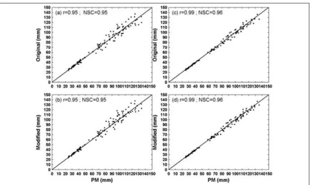
Figure 3. A scatter plot for the estimated vs. the reference values of monthly ET₀at the representative stations: (a-b) for Seoul and (c-d) for Seosan station during the study period

Next, the solar radiations derived from both the original and the modified Angstrom equa- tions were applied to compute ET₀ to see how significantly the modified Angstrom equation affects the irrigation schedule or water resources area. Other meteorological forcing parameters, such as air temperature, wind speed, and relative humidity, were set to be identical in computing ET₀; the only source that would differentiate the estimated ET₀ among the alternatives was the different solar radiation input derived from each method.

The PM equation has been selected for a refer- ence here since the PM equation showed excel- lent performance under a variety of climatic con- ditions, and the FAO-56 PM (hereinafter called FAO PM) described the control condition against which the calibration methods were assessed as

in many other studies (Trajkovic, 2007; Gavilan et al, 2006; Vanderlinden et al., 2004; Irmak et al., 2003a, b; Allen et al, 1998; Allen and Brockway, 1983; Gunston and Batchelor, 1983).

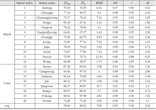
Figure 3 presents the scatter plots for the esti- mated versus the reference values of monthly ET₀ at the representative stations. It was found that there is no noticeable difference between two methods. Table 2-3 presents the monthly esti- mates for the ET₀and its basic statistics. There is some suggestion that the difference is larger in some inland areas because it appears that inland areas are less windy as shown in table 1 and larger portion of ET₀stems from solar radiation in inland areas. The RMSE (AE) is 5.96 (1.75) for the original equation, while it was 5.96 (2.02) for the modified equation. The NSC (r) is 0.95 (0.93) for the original equation, while it was 0.95 (0.93)

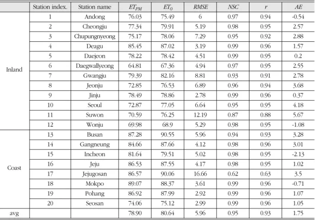
Table 2. The monthly estimates of the ET₀and the corresponding basic statistics for the original Angstrom equation (in mm)

Station index. Station name ET_PM ET₀ RMSE NSC r AE

1 Andong 76.03 75.49 6 0.97 0.94 -0.54

2 Cheongju 77.34 79.91 5.19 0.98 0.95 2.57

3 Chupungnyeong 75.17 78.06 7.29 0.95 0.92 2.88

4 Deagu 85.45 87.02 3.19 0.99 0.96 1.57

5 Daejeon 78.22 78.42 4.51 0.99 0.95 0.2

Inland 6 Daegwallyeong 64.81 67.36 4.94 0.97 0.95 2.55

7 Gwangju 79.39 82.16 8.81 0.93 0.91 2.78

8 Jeonju 72.85 76.53 6.89 0.96 0.94 3.68

9 Jinju 78.49 78.86 2.78 0.99 0.96 0.37

10 Seoul 72.87 77.05 6.64 0.95 0.95 4.18

11 Suwon 70.59 76.25 12.19 0.87 0.88 5.67

12 Wonju 69.98 68.9 5.29 0.98 0.95 -1.08

13 Busan 87.28 90.55 5.96 0.94 0.93 3.28

14 Gangneung 84.66 87.66 4.12 0.98 0.96 3.01

15 Incheon 81.64 79.51 5.02 0.98 0.95 -2.13

Coast 16 Jeju 86.53 87.55 4.17 0.98 0.95 1.02

17 Jejugosan 86.57 90.06 16.66 0.62 0.63 3.5

18 Mokpo 89.07 88.37 3.61 0.99 0.96 -0.71

19 Pohang 86.92 87.99 2.92 0.99 0.96 1.07

20 Seosan 74.06 75.12 2.99 0.99 0.96 1.05

avg 78.90 80.64 5.96 0.95 0.93 1.75

Station index. Station name ET_PM ET₀ RMSE NSC r AE

for the modified equation. The corresponding results are shown in Table 2-3 and Figure 3. It was generally found that both methods show a similar level of performance and that agreement varied with different stations.

Figure 4 shows the monthly performance for both the reference and the estimated ET₀ at the

Figure 4. Relative comparison of basic statistics for the ET₀ derived from two radiation methods: original and modified Angstrom equation

Figure 5. Monthly performance for the estimated ET₀at the representative stations; (a) for Seoul and (b) for Seosan station during the study period.

Table3. The monthly estimates of the ET₀and the corresponding basic statistics for the modified Angstrom equation (in mm)

Station index. Station name ET_PM ET₀ RMSE NSC r AE

1 Andong 76.03 76.05 6.04 0.97 0.94 0.02

2 Cheongju 77.34 80.37 5.4 0.98 0.95 3.02

3 Chupungnyeong 75.17 78.23 7.16 0.95 0.93 3.05

4 Deagu 85.45 87.31 3.34 0.99 0.96 1.86

5 Daejeon 78.22 78.84 4.3 0.99 0.95 0.62

Inland 6 Daegwallyeong 64.81 67.17 4.43 0.98 0.95 2.36

7 Gwangju 79.39 82.75 9.05 0.93 0.91 3.36

8 Jeonju 72.85 77.04 7.02 0.96 0.94 4.19

9 Jinju 78.49 79.22 3.03 0.99 0.96 0.73

10 Seoul 72.87 77.81 7.24 0.95 0.95 4.94

11 Suwon 70.59 76.74 12.54 0.86 0.88 6.16

12 Wonju 69.98 69.67 4.75 0.98 0.95 -0.31

13 Busan 87.28 90.63 5.68 0.94 0.94 3.36

14 Gangneung 84.66 87.53 4 0.98 0.96 2.88

15 Incheon 81.64 79.83 4.84 0.98 0.95 -1.81

Coast 16 Jeju 86.53 87.55 4.09 0.98 0.95 1.02

17 Jejugosan 86.57 89.87 16.7 0.62 0.62 3.3

18 Mokpo 89.07 88.35 3.7 0.99 0.96 -0.72

19 Pohang 86.92 87.98 2.81 0.99 0.96 1.06

20 Seosan 74.06 75.46 3.09 0.99 0.96 1.4

avg 78.90 80.92 5.96 0.95 0.93 2.02

Station index. Station name ET_PM ET₀ RMSE NSC r AE

representative station. The estimates from both alternatives were similar in their seasonal pat- terns. It appeared that the largest difference occurred during summer months for both alter- natives. Previous research (Bois et al., 2008;

McVicar et al., 2007; Gong et al., 2006) has shown that the sensitivity of the climatic variables to ET₀ varies with season and region, and ET₀is mainly governed by solar radiation during summer and by wind speed during winter. In accordance with

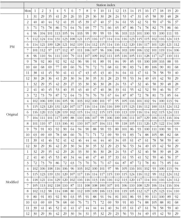
Table 4. The monthly average values of theat each station (in) Station index

1 2 3 4 5 6 7 8 9 10 11 12 13 14 15 16 17 18 19 20

31 29 35 41 29 26 33 29 36 30 28 24 53 47 31 45 58 39 48 28 40 40 44 52 41 35 45 39 47 40 37 34 61 55 42 51 59 47 56 37 71 73 78 86 73 64 76 69 77 71 66 65 87 86 74 78 82 75 86 66 96 104 101 113 105 94 103 99 99 99 93 96 103 113 101 100 93 100 111 93 112 124 114 131 123 108 121 115 116 117 114 114 116 123 115 115 102 116 124 113 114 121 109 128 121 102 119 114 112 115 114 116 112 120 116 117 101 120 121 112 101 112 97 117 112 87 111 106 107 96 106 106 103 109 106 132 101 119 114 106 96 110 94 111 110 79 111 107 109 102 111 105 116 105 111 128 117 127 110 111 78 92 80 92 92 62 96 90 91 89 91 84 99 85 93 100 109 103 88 93 60 68 69 77 69 60 76 70 72 71 68 61 90 83 74 89 106 90 81 68 38 41 45 50 41 41 47 43 45 43 40 34 64 61 47 61 78 58 59 40 30 28 36 41 29 30 34 30 35 31 28 23 55 53 34 49 65 42 50 29 32 29 35 42 29 27 33 30 36 30 28 24 53 47 32 46 58 39 48 28 41 40 45 53 40 35 43 40 47 40 38 33 61 55 42 52 59 46 56 37 72 73 79 87 72 64 73 70 76 70 67 64 87 87 72 78 81 73 85 64 102 106 109 116 105 96 103 102 100 101 97 95 105 116 101 102 94 100 113 94 115 123 120 131 120 107 117 116 114 116 116 109 115 123 116 112 100 113 124 112 116 120 113 128 119 102 115 114 112 115 115 110 113 119 116 114 102 115 124 111 104 111 101 117 109 88 110 106 107 99 106 100 106 111 107 129 106 113 116 104 101 110 97 113 106 81 110 107 107 104 111 99 118 105 111 126 125 122 114 109 79 91 83 92 90 64 94 90 88 90 93 80 101 86 93 100 111 100 90 91 63 69 69 78 68 60 76 71 71 72 69 59 91 83 74 88 105 88 82 68 39 41 46 52 41 42 46 44 44 44 40 34 65 61 47 61 78 58 59 40 30 29 36 42 29 30 34 30 35 32 29 23 56 53 34 49 65 42 50 29 32 29 35 42 29 26 33 30 36 30 28 24 53 47 32 46 58 39 48 28 41 40 45 53 40 34 44 40 47 40 37 33 61 55 41 52 59 46 56 37 72 73 79 86 72 63 73 70 76 71 67 64 87 87 72 78 81 73 85 64 102 106 108 116 106 96 103 102 100 101 97 96 105 116 101 102 93 100 113 94 115 123 119 131 120 107 117 116 114 117 115 110 115 124 116 112 99 112 124 112 118 121 114 129 120 102 116 116 113 116 116 112 113 120 117 114 101 116 124 112 105 113 102 118 110 87 111 108 108 100 107 101 106 110 108 129 106 114 116 104 102 112 98 114 108 80 112 109 109 106 113 101 119 105 112 127 125 123 114 110 80 91 83 92 90 63 95 91 88 91 94 81 101 86 93 99 111 100 89 92 63 69 69 78 68 60 76 71 71 72 69 59 91 83 74 88 105 88 81 68 39 41 46 52 41 41 47 44 44 44 40 34 65 61 47 61 78 58 59 40 30 29 36 42 29 30 34 31 35 32 29 23 56 53 34 49 65 42 50 29

Station index Mon

1 2 3 4 5

PM 6

7 8 9 10 11 12 1 2 3 4 5 Original 6 7 8 9 10 11 12 1 2 3 4 5 Modified 6 7 8 9 10 11 12

that work, Figure 5 presents the seasonal varia- tion in ET₀ estimates with the largest difference occurs during summer season. Table 4 presents the monthly average of ET₀ estimated from two alternatives. It was shown that the difference for the two methods was up to ~2% during the summer season.

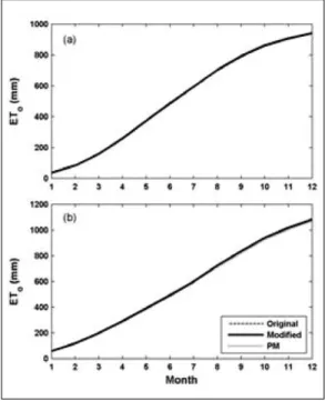
Figure 6 shows a relative comparison of the

annual evolution of the cumulative ET₀according to both alternatives at the representative stations.

There was no prominent difference between the alternatives. The difference for the cumulative ET₀ was not remarkable for either the inland areas or the coastal areas.

The figure shows the exceedance probability (EP) of upper/lower quantiles of the estimated ET₀for a range of confidence level probability.

A statistical evaluation of the estimated ET₀ against the reference values is presented in Figure 7. Figure 7 shows the exceedance proba- bility (EP) of upper/lower quantiles for the esti- mated ET₀for a range of confidence level proba- bility. Both stations showed a similar level of sta- tistical accuracies for the suggested method, mod- ified Angstrom equation. Both sites were associat- ed with high EP values that ranged from near 100% at a high value of CI (0.5) to 60% at 0.1 of CI. It is obvious based on these findings that the modified Angstrom equation provided better per- formance than the original Angstrom equation at each station.

On the basis of the results above, it appears that the two alternatives present a similar level of performance and the modified Angstrom equa- tion is not able to provide any superiority to the original equation in computing ET₀. The modi- fied equation shows better accuracy at some sta- tions, while the original equation shows better accuracy at other stations. These findings may imply that performance varies with region.

V. SUMMARY AND CONCLUSIONS

This paper is based on the previously accepted fact that the nonlinear relationship is more accu- rate than the conventional linear relationship Figure 6. Relative comparison of the annual evolution of

cumulative ET₀according to both alternatives at the representative stations: (a) for Seoul and (b) for Seosan station during the study period

Figure 7. A statistical evaluation of the estimated ET₀ against the reference ET₀.

between solar radiation and bright sunshine duration. The estimation method of solar radia- tion applies to the ET₀. The probable impact of the nonlinear relationships between the solar radiation and bright sunshine duration on the ET₀in irrigation and water resources was thus examined for relative comparison using the con- ventional linear method. The relative accuracies of the different methods are assessed by a com- parison to the reference values. It appears that the two alternatives discussed here present a sim- ilar level of performance, and the difference between the original Angstrom equation and the modified Angstrom equation does not provide the benchmark control that would be desirable to demonstrate a significant difference for the meth- ods. This study suggests that the selection of method used for estimating solar radiation from bright sunshine duration may have a minor influence on estimating ET₀regardless of linearity once the method is locally calibrated, but much attention does need to be paid during summer season because solar radiation dominates ET₀ during the summer season in relative terms.

Acknowledgements

The study is supported by the KORDI project (PE-9853D). The author would like to thank Korea Meteorological Administration (KMA) for their kind cooperation and data provision.

References

Allen, R.G., 1995. Evaluation of procedure for estimating mean monthly solar radiation from air temperature, Report of the Food and Agriculture Organization

(FAO) of the United Nations.

Allen, R.G., 1996. Assessing integrity of weather data for reference evapotranspiration estimation, Journal of Irrigation and Drainage Engineering-ASCE, 122(2), 97- 106.

Allen, R.G., 1997. Self-Calibrating Method for Estimating Solar Radiation from Air Temperature, Journal of Hydrologic Engineering, 2(2), 56-67.

Allen, R.G. and Brockway, C.E., 1983.

Estimating consumptive use on a statewide basis, Proceedings of 1983 Irrigation and Drainage Specialty conference, ASCE, New York

Angstrom, A., 1924. Solar and Terrestrial radiation, Quarterly Journal of Royal Meteorological Society, 50, 121-125.

Annear, R.L., Wells, S.A., 2007. A comparison of five models for estimating clear-sky solar radiation, Water Resources Research 43, W10415, doi:10.1029/2006WR005055.

Bois, B., Pieri, P., Leeuwen, C.V., Wald, L., Huard, F., Gaudillere, J.P., and Saur, E., 2008. Using remotely sensed solar radiation data for reference evapotranspiration estimation at a daily time step, Agricultural and Forest Meteorology, 148, 619-630.

Brustaert, W. 1991. Evaporation into the atmosphere, theory, history and application, Kluwer Academic Publishers, Dordrecht, The Netherland.

Doorenbos, J., Pruitt, W.O. 1977. Guideline for predicting crop water requirements, FAO Irrigation and Drainage Paper 24.

Dorvlo, A.S.S. and Ampratwum, D.B., 2000.

Harmonic analysis of global irradiation,

Renewable Energy, 20, 435-443.

Duan, Q.Y., Gupta, V.K., and Sorooshian, S., 1993. Shuffled complex evolution approach for effective and efficient global minimization”, J. of Optimization Theory and Applications, 76, 501?521.

Duan, Q.Y., Sorooshian, S., and Gupta, V.K., 1994. Optimal use of the SCE-UA global optimization method for calibrating watershed models, Journal of Hydrology, 158, 265-284.

Gavilan, P., Lorite, I. J., Tornero, L. S., and Berengena, J., 2006. Regional calibration of HE for estimating reference ET in a semiarid environment, Agricultural Water Management, 81, 257-281.

Gong, L., Xu, C., Chen, D., Halldin, S., and Chen, Y.D., 2006. Sensitivity of the Penman- Monteith reference evapotranspiration to key climatic variables in the Changjiang (Yangtze River) basin, Journal of Hydrology, 329, 620-629.

Gopinathan, K.K., 1988. A general formula for computing the coefficients of the correlation connecting global solar radiation to sunshine duration, Solar energy, 41(6), 499-502.

Gunston, H. and Batchelor, C. H., 1983. A comparison of the Priestly-Taylor and Penman methods for estimating reference crop evapotranspiration in tropical countries, Agricultural Water Management, 6, 65-77.

Hargreaves, G.L., Hargreaves, G.H., and Riley, P., 1985. Irrigation water requirement for Senegal River Basin, Journal of Irrigation and Drainage Engineering- ASCE, 111, 265-275.

Hay, J.E., 1979. Calculation of monthly mean solar radiation for horizontal and inclined surfaces, Solar Energy, 23(4), 435-443.

Irmak, S., Allen, R.G., and Whitty, E.B., 2003(a). Daily grass and alfalfa- reference-Evapotranpiration calculations as part of the ASCE standardization effort, Journal of Irrigation and Drainage Engineering-ASCE, 129(5), 360-370.

Irmak, S., Irmak, A., Allen, R.G., and Jones, J.W., 2003(b). Solar and net radiation- based equations to estimate reference evapotranspiration in humid climates”, Journal of Irrigation and Drainage Engineering-ASCE, 129(5), 336-347.

Irmak, S., Irmak, A., Jones, J. W., Howell, T.

A., Jacobs, J. M., Allen, R. G., and Hoogenboom, G., 2003(c). Predicting daily net radiation using minimum climatotlogical data”, Journal of Irrigation and Drainage Engineering-ASCE, 129(4), 256-269.

Lee, K., 2009(a). Predicting incoming solar radiation and its application to radiation-based equation for estimating reference evapotranspiration, Journal of Irrigation and Drainage Engineering- ASCE, 135(5), 609-619.

Lee, K., 2009(b). Constructing a nonlinear relationship between incoming solar radiation and bright sunshine duration, International Journal of Climatology, DOI:10.1002/joc.2032

Maidment, D.R., 1993. Handbook of Hydrology, McGraw-Hill, INC., NY, USA McVicar, T.R., Niel, T.G.V., Li, L., Hutchinson, M.F., Mu, X., and Liu, Z., 2007.

Spatially distributing monthly reference evapotranspiration and pan evaporation considering topographic influences, Journal of Hydrology, 338, 196-220.

Nash, J.E., Sutcliffe, J.V., 1970. River flow forecasting through conceptual models, I-A discussion of principles, Journal of Hydrology, 10, 282-290.

Prescott J., 1940. Evaporation from a water surface in relation to solar radiation, Trans R. Sec. South Australia, 64: 114- 118.

Priestly, C.H.B. and Taylor, R.J. 1972. On the assessment of surface heat flux and evaporation using large-scale parameters, Monthly Weather Review, 100(2), 81-92.

Samani, Z.A. 2000. Estimating solar radiation and evapotranspiration using minimum climatological data, Journal of Irrigation and Drainage engineering-ASCE, 126(4), 265-267.

Supit, I., and van Kappel, R.R., 1988. A simple method to estimate global radiation, Solar Energy, 63, 147-159.

Temegsen, B., Allen, R.G., and Jensen, D.T., 1999. Adjusting temperature parameters to reflect well-watered conditions, Journal of Irrigation and Drainage Engineering-ASCE, 125(1), 26-33.

Trajkovic, S. 2007. Hargreaves versus Penman- Monteith under humid conditions, Journal of Irrigation and Drainage engineering-ASCE, 133(1), 38-42.

Vanderlinden, K., Giraldez, J.V., and Meirvenne, M.V. 2004. Assessing reference evapotranspiration by the Hargreaves Methods in Southern Spain”, Journal of Irrigation and Drainage Engineering- ASCE, 130(3), 184-191.

최종원고채택 11. 08. 25