Inhomogeneous Helmholtz equation for Water Waves on Variable Depth

for Marine Environmental Engineering

174

비균질 Helmholtz 방정식을 이용한 변동 수심에서의 파랑변형

김효섭^†·장창환 국민대학교 건설시스템공학부

Inhomogeneous Helmholtz equation for Water Waves on Variable Depth

Hyoseob Kim^† and Changhwan Jang

Department of Civil and Environmental Engineering, Kookmin University, Seoul, Korea

요 약

변동 수심에서의 파랑변형을 비균질 Helmholtz 방정식을 이용하여 계산하였다. 포텐셜 함수가 존재한다고 가정하였 으며, 변수분리를 적용하였다. 본 논문에서는 조화파만을 고려하였다. 포텐셜 함수로 구성된 지배방정식을 정수면에 직접 적용하였고, 변동 수심에 대한 비균질 Helmholtz 방정식을 얻었다. 파랑의 진폭과 위상차로 얻어진 복합 포텐 셜 함수의 지배방정식을 실수형 변수로 된 두 방정식으로 분리하였다. 분리된 방정식들은 각각 1차와 2차 상미분 방 정식이며, 이 방정식들을 단순한 형태의 중앙차분 수치기법을 이용하여 차분식으로 변형하였다. 측면 경계조건에서 의 파랑의 진폭, 진폭경사, 그리고 위상경사를 경계면에 적용하여 전방진행방법으로 전 영역에서 해를 구하였다.

Booij의 경사면 있는 저면의 경우와 Bragg의 물결모양이 있는 저면의 경우에 적용하였다. 본 연구로 도출된 비균질 Helmholtz 방정식은 완전 선형방정식 계산 결과, Massel의 수정 완경사 방정식, 그리고 Berkhoff의 완경사 방정식 의 적용 결과와 비교하였으며, 만족스러운 결과를 얻었다.

Abstract − The inhomogeneous Helmholtz equation is introduced for variable water depth and potential func- tion and separation of variables are introduced for the derivation. Only harmonic wave motions are considered.

The governing equation composed of the potential function for irrotational flow is directly applied to the still water level, and the inhomogeneous Helmholtz equation for variable water depth is obtained. By introducing the wave amplitude and wave phase gradient the governing equation with complex potential function is trans- formed into two equations of real variables. The transformed equations are the first and second-order ordinary differential equations, respectively, and can be solved in a forward marching manner when proper boundary val- ues are supplied, i.e. the wave amplitude, the wave amplitude gradient, and the wave phase gradient at a side boundary. Simple spatially-centered finite difference numerical schemes are adopted to solve the present set of equations. The equation set is applied to two test cases, Booij’s inclined plane slope profile, and Bragg’s wavy bed profile. The present equations set is satisfactorily verified against other theories including the full linear equation, Massel’s modified mild-slope equation, and Berkhoff’s mild-slope equation etc.

Keywords: inhomogeneous Helmholtz equation(비균질 Helmholtz 방정식), variable water depth(변동 수심), separation of variables(변수 분리), complex potential function(복합 포텐셜 함수), spatially-centered finite difference numerical scheme(중앙차분 수치기법)

1. INTRODUCTION

Wave equations for harmonic waves with potential function are distinguished by applicability on variable water depth. The

inhomogeneous Helmholtz equation has been used for solving geological wave propagation in inhomogeneous media, see Manolis and Shaw (1997). Hsiao et al. (1998) also simplified the mild-slope equation to the inhomogeneous Helmholtz equa- tion, and treated the variable water depth as modification of

†

Corresponding author: [email protected]

constant water depth by introducing a perturbation method.

The inhomogeneous Helmholtz equation has not often been used for wave transformation over variable water depth, while the homogeneous Helmholtz equation has been widely used for description of wave transformation over uniform depth since it was proposed by Helmholtz.

Wave transformation over sloped sea bed has been described by the mild-slope equation. The “mild slope” has been defined by a slope smaller than 1/3. The mild-slope equation was developed from either the continuity equation or the principle of stationary action with the variational principle.

The starting point of both the Helmholtz equation and the mild-slope equation is the same. Velocity potential function, Φ, is used to describe the irrotational wave motion. The continu- ity of mass flow in the x-z domain is the Laplace equation:

(1)

where x is the horizontal coordinate, and z is the upward ver- tical coordinate, the origin of which is the still sea level. The continuity of mass flow should be satisfied at every point in the computational domain at every instant. Then, the inte- grated continuity equation will also be satisfied at every sec- tion in the computational domain at every instant.

At free surface boundary nonlinear terms of the momentum equation are ignored, and the following condition in a linear form is applied:

(2)

where t is time, g is the acceleration due to gravity. At the bed the following zero fluid flux condition is applied:

(3)

where h is the water depth relative to the still water level, and varies along x. Considering harmonic motions only, variables are assumed to be separated as:

(4) where complex φ is dependent on x only, and complex Ω is dependent on time only as:

(5) where i = , and is the wave angular velocity, and the function Z is assumed to have the following form:

(6)

Then, the bed boundary condition becomes:

(7)

and

(8)

where k₀ is the wave number at deep sea (=w²/g). Then, the free surface boundary condition, Eq. (9), produces the follow- ing dispersion relationship:

(9)

where both k and h are dependent on x, and Z is dependent on both x and z.

If the water depth is uniform, dh/dx is zero, and we obtain the homogeneous Helmholtz equation:

for one-dimensional problems,

or for two-dimensional problems. (10)

where is the gradient vector in the and directions.

Berkhoff (1973) has derived the mild-slope equation for variable water depth problems. The integration of the equation of continuity equation multiplied by an arbitrary weight func- tion at any selected section should be satisfied at every instant.

Berkhoff chose a hyperbolic cosine function as the weight function in the vertical direction to take into account vertical distribution of wave energy flux, and integrated the equation in the same direction. Berkhoff then took the vertical integration process of the equation which is the multiplication of the con- tinuity equation and the weight function, Z of Eq. (6), in the vertical direction, which is:

(11)

Berkhoff made use of Green’s theorem in order to reflect the bed boundary condition in the middle of his derivation of the mild-slope equation. The mild-slope equation has also been proposed in different types of partial differential equation by Radder (1979) and Copeland (1985).

More recently the modified mild-slope equation was pro-

∂

Φ

∂x

--- ∂

Φ

∂z

---

+ = 0

∂Φ ∂z --- g∂

2

Φ

∂t

--- –

=

∂Φ ∂z --- dh

dx ---∂Φ --- ∂x –

=

Φ Re ZφΩ = ( )

Ω = exp ( – iwt ) 1 –

Z coshk z h ( + ) coshkh ---

=

∂φ ∂z --- dh

---∂ Zφ dx ( ) --- ∂x

=

Z z d

–h

∫

= ^k k ----

k

---- tanhkh k =

d

φ dx

--- k +

φ = 0

∇

φ k +

φ = 0

∇

Z ∂

2

Φ

∂x

--- ∂

Φ

∂z

---

⎝ + ⎠

⎛ ⎞ z d

–h

∫

^{= 0}

posed by Massel (1993), and Chamberlain and Porter (1995).

Two time-dependent forms of the modified mild-slope equa- tion were presented by Suh et al. (1997) by using Green’s the- orem and the variational principle. Suh et al.’s equations are transformed into the modified mild-slope equation of Massel when the time-dependent term is replaced by time-invariant term. The modified mild-slope equation is reduced to the mild- slope equation when some higher-order terms of the modified mild-slope equation are turned off. The modified mild-slope equation reproduces more accurate reflection coefficients for Bragg’s test cases than the mild-slope equation with the aid of additional higher-order terms. Kim et al. (2009) adopted another uniform weight function in the vertical direction as follows:

(12)

However, the above equations, the mild-slope equation, mod- ified mild-slope equation, and Kim et al.’s equation, have a common defect that they don’t satisfy the bed boundary con- dition because they explain horizontally propagating mode only, and this discrepancy is passed over to the other vertical mode for perfect satisfaction of the bed boundary condition.

The continuity should be strictly satisfied in every fluid posi- tion within the computational domain including the still water level, because the wave equation is valid from the still water level to the bed level. If we pickup a level instead of integra- tion of the continuity through the water depth, it corresponds to a case that a delta function is chosen as the weight function at the still water level.

We derive the inhomogeneous Helmholtz equation for vari- able water depth in Section 2, and the equation composed of complex potential function is transformed into two other equa- tions composed of real wave amplitude and wave phase gradi- ent function in Section 3. The system of equations is applied to two topographies for comparison with other theories in Sec- tion 4.

2. DERIVATION OF INHOMOGENEOUS HELM- HOLTZ EQUATION FOR WATER WAVES We apply Eq. (3) to the still water level (z = 0). Then,

(13) (14)

Similarly, we obtain the second derivative of the function Z at the still water level as follows:

(15)

The above results are obvious from the fact that is constant along the still water level, i.e. is always unity from its defini- tion, Eq. (6), and its partial derivative and second partial deriv- ative in the axis on the still water level are also zero. Then, we obtain the inhomogeneous Helmholtz equation with vari- able:

(16)

This equation has the same form as Eq. (10), but is avariable in this equation. Eq. (16) can be considered as an extreme view in which 100% of weight is concentrated on the free surface.

Interestingly, Eq. (16) also quite closely reflects the flow characteristics of the short-wave transformation with the help of the consideration of the bathymetric change through the vari- able k in spite of its relatively simple form. Eq. (15) can be extended to a three-dimensional form by including the other horizontal coordinate, y, as:

(17)

Now Eq. (16) satisfies the governing equation, and the free surface boundary condition is satisfied by the dispersion rela- tionship. Here we examine whether the bed boundary condition could be reflected in the governing equation, the inhomoge- neous Helmholtz equation. When the hyperbolic cosine func- tion of Eq. (6) is applied, the left side of the bed boundary condition, Eq. (7), becomes zero, which leads complete zero horizontal and vertical velocities at the bed. The right side of the bed boundary condition, Eq. (7), reads:

(18)

Replacing the second and first differential terms of the gov- erning equation, Eq. (16), by the non-differential term of Eq. (18) repeatedly, we obtain:

(19) (20)

where g₂ includes k(x) and h(x). Since Eq. (18) should always be satisfied, either φ or g2 should be zero. Zero φ constitutes

∂

Φ

∂x

--- ∂

Φ

∂z

---

⎝ + ⎠

⎛ ⎞ z d

–h

∫

^{= 0}

∂Z ∂x

--- ( k z h ( + ) )′sinh k z h ( ( + ) )cosh kh ( ) kh – ( )′cosh k z h ( ( + ) )sinh kh ( ) cosh

( ) kh

---

=

∂Z ∂x

--- z 0 ( = ) 0 =

∂

Z

∂x

--- z 0 ( = ) 0 =

∂

φ

∂x

--- k +

φ = 0

∇

φ k +

φ = 0

d φ

dx --- ktanhkh dh dx ---φ

– g

( k h , )φ

= =

g

( k h , )φ 0 =

g

( )″tanhkh kh kh ( )′

1 cosh

kh ---

+ + ( )′tanhkh kh

+ k

=

a trivial solution. The other equation, g₂=0, composes another relationship between k and h. This new relationship between k and h comes into conflict with the dispersion relationship between k and h derived from the free surface boundary con- dition. Therefore, we convey this mismatch of the mass con- servation at the bed to evanescent modes instead of applying of this bed boundary condition to the horizontally propagating mode. We can also see that the mild-slope equation and the modified mild-slope equation have the same problem as the present equation. Trials have been attempted to incorporate evanescent modes in dealing with wave propagation problems over sloped beds, see Massel (1993). However the evanescent modes are not of main interest of this paper.

As far as the assumptions of cosine hyperbolic distribution function is adopted for Z function, and Eq. (7) is to be perfectly satisfied, then, both the horizontal velocity and the vertical velocity at the bed should be zero, and the final solution becomes inaccurate. At this point we examine whether Kim and Bae’s (2006) complementary mild-slope equation satisfies the bed boundary condition. They introduced a hyperbolic sine function for Z:

(21)

As far as the dispersion relationship is valid, another relation- ship between k and h develops, and the bed boundary condi- tion cannot be satisfied with propagating mode only, either. In summary the mild-slope equations group to date including the mild-slope equation, the modified mild-slope equation, the complementary mild-slope equation, and the present inhomo- geneous Helmholtz equation can comply with the bed bound- ary condition only with the help of the non-propagating evanescent modes.

The one-dimensional versions of both the Helmholtz equa- tion and the previous equations including the mild-slope equa- tion, modified mild-slope equation, and Kim et al.’s equation can be arranged in the following form:

(22)

While A, B, or C are non-zero functions in the mild-slope equation, modified mild-slope equation, or Kim et al.’s (2009) equation, A, B, and C are zero in the inhomogeneous Helmholtz equation.

Here we introduce two real functions, the wave amplitude, a, the wave phase function, S. And, b is defined as the spatial gra-

dient of the wave phase function as:

and (23)

The wave amplitude and wave phase function are dependent on x for one-dimensional problems. Then, Eq. (16) is split into the following two equations as:

(24)

and

(25) 3. NUMERICAL SOLUTION

A set of real Eqs. (24) and (25) for wave transformation prob- lems over mild-sloped beds are solved. We adopt explicit finite difference schemes for Eqs. (24) and (25). First, Eq. (24) is dis- cretized as:

(26)

and Eq. (25) is discretized as:

(27)

Boundary conditions at a side point are needed. Here a, da/

dx, and b at the right end of the computational domain in the x direction are provided. These are discrete values a_M, a_M-1, and bM. The two finite difference equations are alternately solved:

Eq. (26) for ai-1, and Eq. (27) for bi-1. Both difference equa- tions are centered in space, see Fig. 1:

(28)

and

(29)

Z sinhk z h ( + )

sinhkh ---

=

d

φ dx

--- Adh

dx ---dφ

dx --- k

B d

h dx

--- C dh

dx ---

⎝ ⎠ ⎛ ⎞

φ +

+ + + = 0

φ ae =

b dS dx ---

=

∂

a

∂x

--- + ( k

– b

) = 0

∂b ∂x --- 2

a ---∂a

∂x ---b

+ = 0

a

– 2a

+ a

∆x

--- + ( k

– b

)a

= 0

b

– b

--- ∆x 4 a (

– a

)

∆x a (

+ a

) ---b

+ b

--- 2

+ = 0

a

1

2 --- 4 2 k [ – (

– b

)∆x

a

– 2a

]

=

b

2 G +

2 G –

---b

=

Fig. 1. Variable numbering system in finite difference equations set.

where

(30)

Eqs. (28) and (29) are solved in a forward progressive man- ner from the right side to the left side.

4. VERIFICATION OF THE INHOMOGENEOUS HELMHOLTZ EQUATION

The new set of equations is applied to a series of profiles used by Booij (1983). The bathymetry is composed of an inclined plane with a variable slope or variable width, B, which connects the two flat beds at off-shore and near-shore sides. A step with a bed of a constant slope separates two flat beds, see Fig. 2. The offshore water depth is 60 cm, the near-shore water depth is 20 cm, and the wave period of the incident waves is 2 s.

The boundary values at the right end of the computation domain are simply provided because only outgoing waves exist at the near-shore end. The wave amplitude, a, at the near-shore boundary is chosen as 0.1 m, and the value of the phase func- tion derivative, b, is given the wave number at the shallow zone. The two dependent variables, a and b, are alternately com- puted by half grid size advancement at each computation of Eqs. (28) and (29) from the near-shore end to the off-shore end.

Computed spatial distribution of the relative wave ampli- tude to the outgoing wave amplitude for a specific plane incli- nation, B = 1 m, is shown in Fig. 3. The wave amplitude shows undulation off-shore side from the inclined plane because of the superposition of the incident and reflected waves.

Computed spatial distribution of the wave phase gradient function for a specific plane slope width of 1 m is shown in Fig. 4. The wave phase gradient function also has undulation off-shore side from the inclined plane because of the superpo- sition of incident and reflected waves in the region.

Reflection coefficient, Kr, can be obtained from the com- puted wave amplitude field from the computed maximum and minimum wave amplitudes, a_max and a_min, at the off-shore flat bed zone, that is:

(31)

Computed reflection coefficients from the inhomogeneous Helm- holtz equation for Booij’s test profiles are shown in Fig. 5. In general the reflection coefficients of the inhomogeneous Helmholtz equation are close to those of the full linear equa- tion which does not involve separation of variables (Park et al., 1991). The reflection coefficients of the present equation are smaller than those of the mild-slope equation or the modified mild-slope equation for inclined plane of slope between 0.4 and 4. The origin of these discrepancies should be the differ- ences on the weight functions.

For the plane slopes of greater than or equal to 1, which cor- responds to B

≤0.4 m, the computed reflection coefficients from

G

4 a (

– a

)

∆x a (

+ a

) ---

=

K

a

– a

a

+ a

---

=

Fig. 2. Booij’s test step with inclined plane.

Fig. 3. Computed spatial distribution of relative amplitude for Booij’s bed profile of B=1 m.

Fig. 4. Computed spatial distribution of phase gradient for Booij’s

bed profile of B=1 m.

from the full linear equation, while the mild-slope equation and the modified mild-slope equation and Kim et al.’s (2009) equa- tion show quite large gaps from the full linear equation. The reflection coefficients from the full linear equation, the inho- mogeneous Helmholtz present equation, and the modified mild- slope equation are very close for B larger than or equal to 4 m, because the higher order terms become negligible when the bed slope is small.

Next the inhomogeneous Helmholtz equation is applied to Bragg’s bathymetry to examine its applicability for a different bathymetry, see Fig. 6. It has been known that sinusoidal bathym- etry can cause high reflection depending on the ratio between the bed form length and the wave length. The bathymetry is expressed by the following equation:

(32) where h is the water depth in meter, h₁ and h₂ are the off- shore water depths from the bed forms, respectively, and l is the ripple length.

Incident waves propagate in the positive direction. Calling the wave length L, the computed reflection coefficient for 2l/

L = 0.98 from the Helmholtz equation is 0.748, which closely

agrees with 0.752 from the modified mild-slope equation, and 0.745 from Kim et al.(2009)’s equation, while the reflection coefficient of 0.678 from the mild-slope equation is smaller than the other results, see Fig. 7. The gaps between the reflec- tion coefficients from the mild-slope equation and the other equations are non-negligible. It may be too early to conclude that any one equation is superior to the other equations just from these tests over Bragg’s bathymetry because of difficulty in accurate measurements.

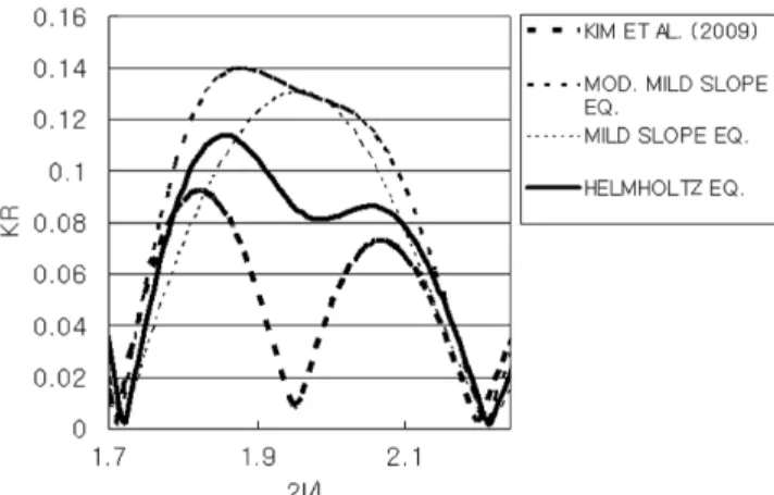
An interesting feature is the distribution of the reflection coefficient around the second resonance point, i.e. 2l/L = 2.

The compared equations produce different reflection coeffi- cients around the point. The computed reflection coefficients from the inhomogeneous Helmholtz equation around the sec- ond resonance point are smaller than those from the mild-slope equation and the modified mild-slope equation, and greater than those from Kim et al.’s equation, see Fig. 8. The explana- tion for this difference could be possible in the future works.

h

= 0.156

h = h

– 0.05sin 2π l⁄ ( ) 0 x 4l ≤ ≤ h

= 0.156

Fig. 5. Comparison of computed reflection coefficients for Booij’s bed profile.

Fig. 6. Bragg’s sinusoidal bathymetry with 4 ripples.

Fig. 7. Comparison of computed reflection coefficients for Bragg’s bed profile.

Fig. 8. Zoomed computed reflection coefficients for Bragg’s bed

profile around second resonance.

5. CONCLUSIONS

The inhomogeneous Helmholtz equation is adopted and examined for description of harmonic wave transformation over variable depth. The continuity equation has a weight of a delta function along the still water level, and is assumed to be sepa- rated by two functions, a vertical distribution function Z, and a spatial potential function Φ in the x axis. The inhomogeneous Helmholtz equation has two forms: a form with the complex velocity potential function, and the other form in a set of equa- tions with the wave amplitude and the wave phase function.

The inhomogeneous Helmholtz was applied to two bed pro- files, Booij’s inclined bed profile, and Bragg’s wavy ripple bed profile. The inhomogeneous Helmholtz equation was verified against other theories.

The test of the present equation on Booij’s steps reveals that the inhomogeneous Helmholtz equation provides better accu- rate reflection coefficient with respect to the solutions from the full linear equation than the modified mild-slope equation or the mild-slope equation. Moreover the inhomogeneous Helm- holtz equation shows good agreement over wide range of bed slopes.

The test of the present equation on Bragg’s sinusoidal rip- ples confirms that the inhomogeneous Helmholtz equation pro- duces correct reflection coefficient when the ripple length is about half of the wave length compared with other theories, e.g. the modified mild-slope equation, and the modified mild-slope equa- tion, or Kim et al.’s (2009) equation.

The numerical experiments over two kinds of bathymetry confirm the accuracy and applicability of the inhomogeneous Helmholtz equation based on the delta weight function along the still water level.

ACKNOWLEDGEMENTS

The work was supported by Korean Ministry of Land, Trans- port and Maritime Affairs, and Korea Institute of Marine Sci- ence & Technology Promotion under the title of “Marine and Environmental Prediction System (MEPS)” in 2009-2010, and by Kookmin University as a university grant in 2010.

REFERENCES

[1] Berkhoff, J.C.W. 1973. Computation of combined refraction-dif- fraction. Proc. 13

Intl. Conf. on Coastal Engineering, July 1972, Vancouver, Canada, pp. 471-490. ASCE.

[2] Booij, N. 1983. A note on the accuracy of the mild-slope equa- tion. Coastal Engineering. 7, 191-203.

[3] Chamberlain, P.G., Porter, D. 1995. The modified mild-slope equation. J. Fluid Mech. 291, 393-407.

[4] Copeland, G.J.M. 1985. A practical alternative to the mild-slope wave equation. Coastal Engineering. 9, 125-149.

[5] Hsiao, S.S., Weng, W.K. and Chiu, Y.F. 1998. Wave forces on a circular island using perturbation - DRBEM. Eighth Interna- tional Offshore and Polar Engineering Conference, Montreal, Canada.

[6] Kim, H., Jung, B. and Lee, Y. 2009. A linear wave equation over mild-sloped bed from double integration. J. Korean Society for Marine Environmental Engineering. 12(3), 165-172.

[7] Kim, J.W., Bai, K.J. 2004. A new complementary mild-slope equation. J. Fluid Mech. 511, 25-40.

[8} Kirby, J.T. 1986. A general wave equation for waves over rippled beds. J. Fluid Mechanics. 162, 171-186.

[9] Luke, J.C. 1967. A variational principle for a fluid with a free sur- face. J. Fluid Mech. 27, 395-397.

[10] Manolis, G.D. and Shaw, R.P. 1997. Fundamental solutions to Helmholtz’s equation for inhomogeneous media by a first-order differential equation system. Soil Dynamics and Earthquake Engineering. 16, 81-94.

[11] Massel, S.R. 1993. Extended reflection-diffraction equation for surface waves. Coastal Engineering. 19, 97-126.

[12] Porter, D., Staziker, D.J. 1995. Extentions of the mild-slope equation. J. Fluid Mech. 300, 367-382.

[13] Park, W.S., Lee, D.S., Oh, Y.M., Jeong, W.M. 1991. Infinite ele- ments for analysis of diffraction and radiation problems in the vertical plane. J. Korean Soc. Coastal Ocean Engineers, 3 (4), 235-243 (in Korean).

[14] Rather, A.C. 1979. On the parabolic equation method for water- wave propagation. J. Fluid Mech. 95, 159-176.

[15] Suh, K.D., Lee, C., Park, W.S. 1997. Time-dependent equations for wave propagation on rapidly varying topography. Coastal Engineering. 32, 91-117.

2010년 5월 28일 원고접수

2010년 7월 1일 심사완료

2010년 7월 1일 수정본 채택