Bayesian Model for Cost Estimation of Construction Projects

(1)

Kim, Sangyong^* ¹⁾

School of Construction Management and Engineering, University of Reading, Reading, RG6 6AW, UK

Abstract

Bayesian network is a form of probabilistic graphical model. It incorporates human reasoning to deal with sparse data availability and to determine the probabilities of uncertain cases. In this research, bayesian network is adopted to model the problem of construction project cost. General information, time, cost, and material, the four main factors dominating the characteristic of construction costs, are incorporated into the model. This research presents verify a model that were conducted to illustrate the functionality and application of a decision support system for predicting the costs. The Markov Chain Monte Carlo (MCMC) method is applied to estimate parameter distributions. Furthermore, it is shown that not all the parameters are normally distributed. In addition, cost estimates based on the Gibbs output is performed. It can enhance the decision the decision-making process.

Keywords : Bayesian, Cost estimating, Markov Chain Monte Carlo

1. Introduction

1.1 Research Background

Successful management of construction project cost within the limited budget is an important concern in any construction project. Lack of information and reliable tools that support estimating process made it difficult to initiate estimating report during the project planning stage[1]. In order to control the cost within an acceptable level, it requires appropriate and accurate measurement of various project related determinants and the understanding of the magnitude of their effects. As such, the importance of early estimating to owners and related project teams cannot be over emphasized.

Several studies have demonstrated focus on cost estimating in the past. Although multiple regression analysis has been used to cost estimating based on

Received : January 20, 2011

Revision received : February 8, 2011 Accepted :February 14, 2011

* Corresponding author : Kim, Sangyong [Tel: , E-mail: ]

statistics many times, it is not appropriate when describing non-linear relationships which are multidimensional, consisting of a multiple input and output problem[2]. Chou et al[3] suggested heuristic simulation models to improve the accuracy and efficiency of budgeting estimates based on useful data from the Texas Department of Transportation (TxDOT). Artificial intelligence (AI) approaches were developed using the expert systems, artificial neural networks (ANNs), and case-based reasoning (CBR) for reasons of its limitation, and the models were demonstrated that they were very useful at the early phases of a project life cycle[4,5,6].

However, the expert system, which use rule-based reasoning, have difficulty in obtaining a correct set of rules that can elicit knowledge in non-experienced komains[7,8] and these systems lack the capability to learn by themselves[8,9]. ANNs can lose their effectiveness when the patterns are very complicated or noisy, ill-defined knowledge representation and problem structuring, and training trapped in local minima[10].

And, CBR has limitation to reflect suitable current criteria to index and match and depending on previous experience without validating it in the new situation[11].

Bayesian networks are a probabilistic graphical model

(2)

that represents a set of random variables and their conditional dependencies via a directed cyclic graph[12].

This research develops a probabilistic framework for cost estimating using a bayesian approach. The body of information that can be used to construct and update the probabilistic models includes objective information. The bayesian approach used in this research is ideally suited for incorporating different sources of information[13]. The prevailing uncertainties, model errors arising from an inaccurate model form or missing variables, measurement errors, and statistical uncertainty are accounted for in the proposed approach.

Especially, bayesian approach has been proposed as effective alternatives to the support of decision making.

Several studies have demonstrated potential applications of bayesian in construction areas. Gardoni et al.[13]

developed a probabilistic framework for forecasting job progress and final time-to-completion. Kim and Reinschmidt[14] focused on the probabilistic schedule forecasting of ongoing projects. Tang and McCabe[15]

approached the development of a method for incomplete data to estimate the whole domain in engineering management decision making. Haas and Einstein[16]

applied bayesian techniques to their developed too, decision aids for tunneling. And, Chung et al.[17]

demonstrated how the statistical distributions of the input parameters are updated using bayesian techniques.

Learning from previous researches and applications bayesian network can overcomes most of the drawbacks of previous methods, and make very resonable estimating without using specific experts and rules. First, it is effective in explaining the procedure for obtaining the cost of a new project, and does not need to utilizes the specific knowledge gained from previous. Second, it does not require extensive analysis of knowledge area. Third, it permits problem solving even if structure of data is incomplete.; the bayesian networks can estimate the cost of a future construction project accurately.

Estimating future construction cost at the preliminary design phase is the focus of this research by total cost.

The paper is organized as follows. The next section describes the objectives methodology of this research. The next section briefly presents the bayesian networks that were developed specifically to generate bayesian

applications for modelling cost estimates and the steps followed in developing an application. The following section shows how this data was analyzed to verify its consistency and completeness and to obtain the knowledge required for the application. Then, thirty-eight actual cases of highway project data constructed in South Korea, from 1996 to 2008, have been used as the source of cost data and in developing a bayesian application for systematic highway project is presented. Finally, the testing procedures and the validation results are discussed.

1.2 Objectives

The major objective of this research is to develop a bayesian decision support model for estimating of a construction project cost based on recent historical project data. Basically, this research has been carried out two things which are extraction of cost significant items (CSIs) in construction projects and development of a bayesian model. The research goals included (1) extract CSIs using the commercial statistical package for the social sciences (SPSS) version 19 for window tool; (2) develop a bayesian model using WinBUGS based on Markov Chain Monte Carlo (MCMC) methods; (3) estimate a highway cost at the early stage of a project by total cost. As a result, the developed model provides a useful benchmark against which bayesian model can be measured, and it assists in identifying those variables that demonstrated a strong relationship with a highway construction cost.

1.3 Methodology

CSIs are very complicated which requires intelligent processing to get a precise view of the effects of the cost attributes on project cost[18]. The data is required that incorporates all the CSIs, the kinds of which are known from previous studies. First of all, this research compiled such as shown in Table 1 summarized literature review and identified 21 CSIs which affect cost of a construction projects. Furthermore, industrial interview were conducted to assist deciding these factors. When potentially CSIs were identified, the CSIs of data were analyzed by SPSS. In addition appropriate bayesian model

(3)

number of data sets.

2. Model Estimation through Bayesian

2.1 Definition of Bayesian

Bayesian network, also known as belief networks, belongs to the family of probabilistic graphical models.

Bayesian network forms an attractive framework in developing normative systems, which are meant to make decisions based on accumulated and processed experiences[19]. It is a very general and powerful tool as seen in previous section that can be used for a large number of problems involving uncertainty: reasoning, learning, planning, and perception. The network consists of a set of variables and a set of directed links between any two variables, it is indicated by a directional arrow leading from the cause variable to the effect variable[20].

The causal relations or links in the network are quantified by assigning conditional probabilistic values to express their strengths. These conditional probabilities are evaluated using the well-known bayesian theory[21].

2.2 Problem Definition

Bayesian inference combines the information from observed data with prior knowledge about the parameters (prior) to arrive at the updated distribution of the parameters (posterior)[22], which is described as

( | , ) ( | ) ( | , ) ( | )

( | , )

( | ) ( | , ) ( | )

p Y X p X p Y X p X

p X Y

p Y X p Y X p X d

ψ ψ ψ ψ

⋅ ⋅

= =

⋅ ⋅

∫

(1) where X=assumed probabilistic model class for the target system; ψ=uncertain model parameters;

Y=measured data from the system; p(ψ|X)=prior probability density function of ψ; p(Y|X,ψ)=likelihood;

and p(Y|X) is called the evidence of X.

The goal of bayesian model class selection is quite different. Given the chosen candidate probabilistic model classes {X⁽ⁱ⁾:i=1,...,Nclass} the goal of bayesian model class selection is to calculate F[X⁽ⁱ⁾|Y]

1

[ | ] [ ]

i

p Y X F X

∑= (2) where F [X⁽ⁱ⁾]=prior probability of X(i). Notice that the calculation of F[X⁽ⁱ⁾|Y] requires the determination of the evidence {p[Y |X⁽ⁱ⁾]:i=1,...,Nclass}. Once bayesian model class selection is achieved, bayesian model averaging is trivial because any quantity of interest g conditioning on the data and all the chosen model classes can be estimated using the following equation:

( ) ( )

1

( | ) ^class [ | , ] [ | ]

N

i i

i

E g Y E g X Y F X Y

=

= ∑ ⋅ (3)

2.4 Posterior

The posterior distribution reflects both the information known a priori, included in the prior distribution, and the objective information included in the likelihood function[13]. It is centered at a point that represents a compromise between the prior information and the data[13]. The compromise is increasingly controlled by the data as the sample size increases[23]. With the prior and likelihood functions at hand, using Eq. (1), the posterior is obtained as

p(ψ|X,Y)

∝ ⁽ ^{| , )} ^{( |} ^{, )} ⁽ ^, ^| ^, ⁾ ^{( | , )}

i

N N u G j j j j G

i j

p β β ∑ p β β Δ p w ϑ ϕ p η φ ς

∏ ∏

(4) where i=section number; ϕ=parameter to be estimated;

βu=mean of β; φ,ς=parameters of the gamma distribution of η; pN(∙|∙)=normal density function; pG(∙|

∙)=gamma density function; wj,j=j,j element of matrix ∑

-1, w j,j∼gamma(ϑj,ϕj); and η=precision of the error term distribution.

As shown in the posterior distribution, there are nine regression parameters to be estimated. Although the joint distribution of these variables conditional on the given data is obtained, the goal is to arrive at the marginal distribution of each variable, which requires the multi-dimensional integration of the right-hand side of Eq. (4). It is apparent that the multi-dimensional integration task for solving Eq. (4) is staggering.

However, an alternative to avoid the complexity in obtaining the marginal distribution is available through

(4)

the Gibbs sampler with MCMC simulation, which is presented in the following section.

2.5 Gibbs Sampling

(1) (0) (0) (0)

1 1 2 3

(1) (1) (0) (0)

2 2 1 3

( | , ,..., )

m m

U from f U U U U U from f U U U U …

(1) (1) (0) (1)

1 2 1

( | , ,..., )

m m m

U from f U U U U ₋ (5) The process of the algorithm used in the Gibbs sampling is described as follows: for a set of random variables U1,U2,...,Um, the joint distribution is denoted as f(U1,U2,...,Um). With given arbitrary starting values of Us's, say U1(0),U2(0w),...,Um⁽⁰⁾, the first iteration of random draws of Us's is obtained. In a similar manner, the second set of random draws of Us^'s is obtained through the update process. After r iterations, the series of Us^'s is obtained as (U1^(r).U2^(r),...,Uk^(r)), which means that after enough iterations, r, U1^(r)can be regarded as a random draw from the distribution of (U1^(r))[24].

Based on the above algorithm, the application of MCMC for obtaining the marginal distribution of each parameter conditional on observed data is straightforward [25,26]. It is shown that the joint distribution by the given data set is available through the Bayesian approach, which is the posterior [Eq. (4)]. With the joint conditional distribution of the parameter set, the MCMC simulation is carried out, leading to the simulated distribution of each parameter of interest[26].

3. Selection of Cost Significant Items

3.1 Construction Costs

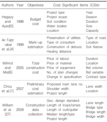
While there are a few studies offered on CSIs that are thought to relate to construction cost, numerous studies have taken place in construction projects as presented in Table 1.

The research of Hegazy and Ayed[5] was based on collected 18 bidding data. The research was worked with ANNs to develop a cost estimating model where little information is known about the scope of the project and Genetic Algorithms (GAs) was used to find the optimum weights of the model. Up to 10 major factors were included in the developed three methods used to

determine optimum ANNs model, and in the best method the developed simplex optimization. Al-Tabtabai et al.[4], and Wilmot and Mei[6] had pursued a similar approach as Hegazy and Ayed[5]. ANN models were developed which relates construction cost to estimate the factors affecting items were used. Still, their CSIs are interesting for the present research, especially considering the not many researches have been done so far about estimating for a construction project.

Chou and O'Connor[1] developed the web-based system so that engineers could use it to estimate preliminary costs with quantity-based models of a construction project at the conceptual phase. In addition, the focus of their research was on a web-based database design and implementation of an information system development.

Table 1. Previous studies and their relevant CSIs Authors Year Objectives Cost Significant Items (CSIs)

Hegazy and Ayed[5]

1998 Budget

cost

Project type Project scope Soil condition Water bodies Location

Year Season Duration Size Capacity Al-Tabt

-abai et al.[4]

1999 Mark-up estimation

Preservation of utilities Type of consultant Construction of detours Hauling distance

Type of road Location Soil Nature

Wilmot and Mei[6]

2005

Total construction

cost

Price of labour Price of material Price of equipment No. of plan changes Change in specification

Duration Location Bid volume Bid variable Contract type Chou

et al.[1] 2007

Preliminary cost estimation

Proposed main lane no.

Shoulder width Project length

Lane width Location

William et al.

[27]

2009

Construction data collection

Geo. design standard Length of loops/ramps Length of curb/gutter Median length/type Project length

Lane length Bridge type Bridge length Bridge width

3.2 Survey Data

The survey questionnaire was designed to enable respondents to add any further variables that they considered necessary for inclusion to the list of related factors. The review of related researches supplies a list of CSIs of a highway project that is further re-examined in expert interviews: architects, cost planners, and cost estimators for construction firms are given the task of

(5)

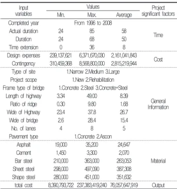
confidence of data was come by step by step selecting procedure as shown in Figure 1. As a fist result further variables show up to be important, for example general information, time, cost, and materials related variables of a highway project. The data of 21 CSIs, derived following the analysis of the initials results, are as presented in the Table 2. It has to be noted that an additional CSIs was excluded from the final list, following the results of the statistical analysis.

The cost of a project

Can cost significant items be extracted?

Extract cost significant items based on published

information

Can cost significant items be extracted?

List all cost significant items

Check first decided cost significant items

Available?

Acceptable?

Check other cost significant items

Gather all acceptable and available cost significant items

as a candidate set up

End Yes

No

Yes

No No

Yes

Yes All cost significant

items done?

No Find the set of available cost

significant items strongly related to this project using expert interview

Check first cost significant items

Available?

All cost significant items done?

All cost significant items done under this

environment

Check other cost significant items Experts add/remove

decided cost significant items compare with real- world information and

data No

No

No Yes

Yes

Yes SPSS Analysis

Figure 1. Selecting Procedure of CSIs

variables Min. Max. Average significant factors Completed year From 1996 to 2008

Actual duration 24 85 58 Time

Duration 24 68 50

Time extension 0 36 8

Design expenses 239,137,621 6,371,670,030 2,161,041,843 Contingency 310,459,368 8,568,800,000 2,815,219,944 Cost Type of site 1.Narrow 2.Medium 3.Large

General Information Project scope 1.New 2.Rehabilitation

Frame type of bridge 1.Concrete 2.Steel 3.Concrete+Steel Length of highway 3.34 49.00 8.39

Ratio of ridge 0.30 9.80 1.68

Wide of Highway 23.4 37.8 26.7

Wide of bridge 2.6 28.4 15.4

No. of lanes 4 8 5

Pavement type 1.Concrete 2.Ascon

Asphalt 19,000 35,200 24,647

Material

Cement 1,450 3,300 2,070

Bar steel 210,000 363,000 263,053 Sheet steel 298,000 497,090 387,308 Shape steel 280,000 451,000 351,632

total cost 8,390,793,722 237,383,419,240 76,057,647,919 Output

3.3 Data Analysis Using Regression Technique

A multiple regression analysis was conducted using SPSS to evaluate how the factors influenced cost estimating. The independent factors were 21 CSIs identified in the previous section.

The linear combination of these items was significantly related to the production per shift, F(9.23)=8.491, p <

.001, indicating that the explained variance by the regression equation is large compared to the unexplained factors. Table 3 shows the coefficients for each item and the statistical results of the regression model.

To analysis the relative importance of those factors affecting the cost estimating, the unstandardized coefficients were multiplied for each statistically significant factor from the regression model.

Table 3. Coefficient of regression model Model B Beta t Sig.

(Constant) 570.739 - 1.982 .057

Completed year -.284 -.224 -1.952 .061

Duration (m) -.023 -.084 -1.598 .121

Time extension (m) .035 .075 1.451 .158

Design expenses .002 .618 3.050 .005

Contingency .001 .409 2.090 .046

Type of site -.283 -.035 -1.552 .132

Cement (won/kg) 6505.989 1.017 3.635 .001

Bar steel (won/kg) -99.233 -1.261 -4.051 .000

Shape steel (won/kg) 32.374 .425 1.683 .103

(6)

4. Fitting Bayesian Model

4.1 Introduction to WinBUGS

WinBUGS (the MS Windows operating system version of BUGS: Bayesian Analysis Using Gibbs Sampling) is a versatile package that has been designed to carry out MCMC computations for a wide variety of bayesian models. WinBUGS implements various MCMC algorithms to generate simulated observations from the posterior distribution of the unknown quantities in the statistical model. The idea is that with sufficiently many simulated observations, it is possible to get an accurate picture of the distribution.

4.2 Model Development

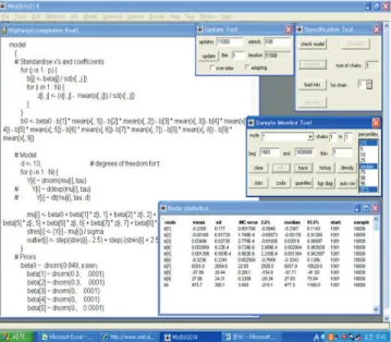
Figure 2. Bayesian model interactively in WinBUGS

To run the model, the author sets the 󰡒Specification Tool󰡓󰡒Sample Monitor Tool󰡓and 󰡒Update Tool󰡓as shown in Figure 2. In the first step, the model is selected the syntax, loading the data, compiling the model, and loading initial values by highlighting keyword in the appropriate input files. The next phase is needed samples retained for output analysis. The last tool is then used to request the number of iterations to be run. The coding source of bayesian is opened in Figure 3.

model {

# Standardise x's and coefficients for (j in 1 : p) {

b[j] <- beta[j] / sd(x[ , j ]) for (i in 1 : N) {

z[i, j] <- (x[i, j] - mean(x[, j])) / sd(x[ , j]) }

}

b0 <- beta0 - b[1] * mean(x[, 1]) - b[2] * mean(x[, 2]) - b[3] * mean(x[, 3])- b[4] * mean(x[, 4]) - b[5] * mean(x[, 5]) - b[6] * mean(x[, 6])- b[7] * mean(x[, 7]) - b[8] * mean(x[, 8]) - b[9] * mean(x[, 9])

# Model

d <- 10; # degrees of freedom for t

for (i in 1 : N) {

Y[i] ~ dnorm(mu[i], tau)

# Y[i] ~ ddexp(mu[i], tau)

# Y[i] ~ dt(mu[i], tau, d)

mu[i] <- beta0 + beta[1] * z[i, 1] + beta[2] * z[i, 2] + beta[3] * z[i, 3] + beta[4] * z[i, 4] + beta[5] * z[i, 5] + beta[6] * z[i, 6] + beta[7] * z[i, 7] + beta[8] * z[i, 8] + beta[9] * z[i, 9]

stres[i] <- (Y[i] - mu[i]) / sigma

outlier[i] <- step(stres[i] - 2.5) + step(-(stres[i] + 2.5) ) }

# Priors

beta0 ~ dnorm(0.049, 0.0001)

beta[1] ~ dnorm(0.3, .0001)

beta[2] ~ dnorm(0.3, .0001)

beta[3] ~ dnorm(0, .0001)

beta[4] ~ dnorm(0, .0001)

beta[5] ~ dnorm(0., 0.0001)

beta[6] ~ dnorm(0, 0.0001)

beta[7] ~ dnorm(-100, 0.0001)

beta[8] ~ dnorm(-100, 0.0001)

beta[9] ~ dnorm(0, 0.0001)

tau ~ dgamma(1.0E-3, 1.0E-3) phi ~ dgamma(1.0E-2,1.0E-2)

# standard deviation of error distribution

sigma <- sqrt(1 / tau) # normal errors

# sigma <- sqrt(2) / tau # double exponential errors

# sigma <- sqrt(d / (tau * (d - 2))); # t errors on d degrees of freedom

Figure 3. Coding source of bayesian model 4.3 Analyzing the Output

Figure 4. Trace of each CSI

(7)

sufficient iterations have been run. The script in the analysis file sets up and samples it for 10,950. A total sample of 10,900 is used for summarization and convergence checks after discarding the first 10,850 burn-in iterations as shown in Figure 4.

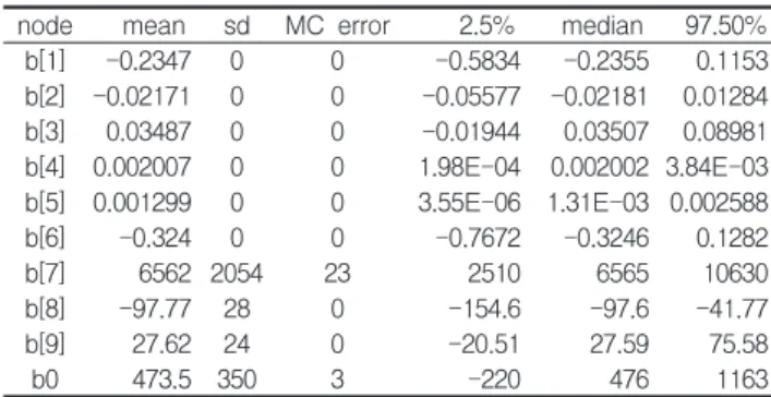
Among the available options for summarizing these estimated posterior distributions are density plots (smoothed kernel density plots for continuous quantities and bar graphs for discrete ones; see Figure 5) and tabular summaries (see Table 4).

Table 4. Node statistics

node mean sd MC error 2.5% median 97.50%

b[1] -0.2347 0 0 -0.5834 -0.2355 0.1153

b[2] -0.02171 0 0 -0.05577 -0.02181 0.01284

b[3] 0.03487 0 0 -0.01944 0.03507 0.08981

b[4] 0.002007 0 0 1.98E-04 0.002002 3.84E-03

b[5] 0.001299 0 0 3.55E-06 1.31E-03 0.002588

b[6] -0.324 0 0 -0.7672 -0.3246 0.1282

b[7] 6562 2054 23 2510 6565 10630

b[8] -97.77 28 0 -154.6 -97.6 -41.77

b[9] 27.62 24 0 -20.51 27.59 75.58

b0 473.5 350 3 -220 476 1163

The columns of Table 4 represent the node name; the estimated mean and standard deviation of the posterior distribution; he autocorrelation-adjusted standard error of the estimated posterior mean; the 2.5%, 50%, and 97.5% quantiles of the posterior distribution.

Figure 5. Posterior density plot

used for performance evaluation. The performance of bayesian model was measured by the mean absolute error rate (MAER), which was calculated by Eq. (6).

( | ^e ^a 100 |)

a

C C MAER C

n

− ×

= ∑

(6) where Ce is the estimated construction costs, Ca is the collected actual construction costs, and n is the number of test data.

Table 5. Predicting result of bayesian model Case Actual cost

(million won)

Estimated cost Error rate (%) Posterior Non-

posterior Posterior Non- posterior

1 21,959 23,256 24,898 5.91 13.38

2 43,997 45,403 47,001 3.20 6.83

3 66,572 69,108 70,700 3.81 6.20

4 159,486 164,322 165,899 3.03 4.02

5 76,252 80,484 82,100 5.55 7.67

MAER 4.30 7.62

A comparison of the predicting result with the development of the bayesian model, posterior and non posterior, shows following:

The performance of the bayesian posterior model was somewhat superior to that of the non-posterior model as shown in Table 5. The best result in posterior was obtained that the error rate is 3.03%, whereas the average result is calculated 4.30% from the bayesian posterior model. In the decision-making process, Bayesian posterior model is considered quite an appropriate method in explaining the procedures for obtaining the cost of a new project at the preliminary design phase. Accordingly, decision-maker can apply the Bayesian posterior model to estimate any construction project costs with uncertainty.

5. Conclusions

Since construction cost is affected by many uncertainties, tools for decision-making under uncertainty are needed. This research suggests using bayesian models to the distributions of input parameters

(8)

for construction project cost. The model accounts for the fundamental factors associated with construction project cost: General information, time, cost, and material.

Regression analysis based on the actual collected project data was first conducted to identify the factors affecting the productivity. The results show that items such as the table 3, As a result, those are significantly affected construction project cost.

The bayesian posterior is obtained by updating the prior with the observed data and reflects the characteristics of the actual CSIs. The Gibbs sampling algorithm is used to estimate the distributions of the individual parameters. As a result, although the methodology presented in this research is aimed at developing probabilistic bayesian model to predict construction cost, the approach is quite general and can be used for forecasting in other application in construction areas. Following the philosophy of bayesian updating, the research approach presented in this research can be applied to enhance the current model as new data are collected.

However, one problem is that different user can have different estimation on the probability of the case featured in the proposed model. Different project managers even on the same project may have different evaluations based on their own judgement. Therefore, future research could incorporate a group decision module in the model to collect input on the conditional probabilities of CSI relationships and the relative weights between different project CSIs from a group of experts rather than one. Such a group decision module would increase the efficiency and accuracy of the input and therefore the results.

References

1. Chou JS, O'Connor JT. Internet-Based Preliminary Highway Construction Cost Estimating Database. Automation in Construction 2007;17(1):65-74.

2. Tam CM, Fang CF. Comparative Cost Analysis of Using High Performance Concrete in Tall Building Construction by Artificial Neural Networks. Structural Journal 1999;96(6):927-936.

3. Chou JS, Wang L, Chong WK, O'Connor JT. Preliminary Cost

Estimates Using Probabilistic Simulation for Highway Bridge Replacement Projects. ASCE Proceeding of the Congress 2005.

4. Al-Tabtabai H, Alex AP, Tantash M. Preliminary Cost Estimation of Highway Construction Using Neural Networks.

Cost Engineering 1999;41(3):19-24.

5. Hegazy T, Ayed A. Neural Network Model for Parametric Cost Estimation of Highway Projects. Journal of Construction Engineering and Management 1998;124(3):210-18.

6. Wilmot CG, Mei B. Neural Network Modelling of Highway Construction Costs. Journal of Construction Engineering and Management 2005;131(7):765-71.

7. Watson I. Applying Case-Based Reasoning: Techniques for Enterprise Systems. 1st Ed. Morgan Kaufmann Publishers Inc.; 1997.

8. An SH, Kim GH, Kang KI. A Case-Based Reasoning Cost Estimating Model Using Experience by Analytic Hierarchy Process. Building and Environment 2007;42(7):2573-79.

9. Yau NJ, Yang JB. Case-Based Reasoning in Construction Management. Computer-Aided Civil and Infrastructure Engineering 1998;13(2):143-50.

10. Hegazy T, Fazio P, Moselhi O. Developing Practical Neural Network Applications Using Back-Propagation.

Computer-Aided Civil and Infrastructure Engineering 1994;9(2):145-59.

11. Kolodner JL. An Introduction to Case-Based Reasoning.

Artificial Intelligence Review 1992;6(1):3-34.

12. Wikipedia. Bayesian Network. http://en.wikipeda.org/ wiki/

Bayesian_network 2010.

13. Gardoni P, Reinschmidt KF, Kumar R. A Probailistic Framework for Bayesian Adaptive Forecasting of Project Progress. Compter-Aided Civil and Infrastructure Engineering 2007;22(3):182-96

14. Kim BC, Reinschmidt KF. Probabilistic Forecasting of Project Duration Using Bayesian Inference and the Beta Distribution. Journal of Construction Engineering and Management 2009;135(3):178-86.

15. Tang Z, McCabe B. Developing Complete Conditional Probability Tables from Fractional Data for Bayesian Belief Networks. Journal of Computing in Civil Engineering 2007;21(4):265-276.

16. Haas C, Einstein HH. Updatng the Decision Aids for Tunneling. Journal of Construction Engineering and Management 2002;128(1):40-48.

17. Chung TH, Mohamed Y, AbouRizk S. Bayesian Updating

(9)

and Management 2006;132(8):882-94.

18. Boussabaine AH, Elhag TMS. Knowledge Discovery in Residential Construction Project Cost Data. 15th Annual ARCOM Conference 1999:489-98.

19. Jensen FV. Bayesian Networks and Decision Graphs. 2nd Ed. USA, New York:Springer; 2007.

20. Naidu ASK, Soh CK, Pagalthivarthi KV. Bayesian Network for E/M Impedance-Based Damage Identification. Journal of Computing in Civil Engineering 2006;20(4):227-36.

21. Montgomery DC, Runger GC. Applied Statistics and Probability for Engineers, 4th Ed. USA, New York:Wiley;

2006.

22. Zellner A. An Introduction to Bayesian Inference in Econometrics. 2nd Ed. New York;Wiley; 1996.

23. Box GEP, Tiao GC. Bayesian Inference in Statistical Analysis. 1st Ed. New York;Wiley;1992.

24. Geman S, Geman D. Stochastic Relaxation, Gibbs Distributions and the Bayesian Restoration of Images, IEEE Transactions on Pattern Analysis and Machine Intelligence 1984;6(6):721-41.

25. Brooks SP. Markov Chain Monte Carlo Method and Its Application. Journal of the Royal Statistical Society, Series D 1998;47(1):69-100.

26. Hong F, Prozzi JA. Updating Pavement Deterioration Models Using the Bayesian Principles and Simulation Techniques.

1st Annual Inter-University Symposium on Infrastructure Management 2005.

27. Williams RC, Hildreth JC, Vorster MC. Journal of Construction Engineering and Management 2009;135(12):1299-1306.