Estimation of stream flow discharge using the satellite synthetic aperture radar images at the mid to small size streams
Seo, Minji
aㆍKim, Dongkyun
a*ㆍAhmad, Waqas
aㆍCha, Jun-Ho
ba
Department of Civil Engineering, Hongik University
b
Han River Flood Control Office, Ministry of Environment
Paper number: 18-060
Received: 2 August 2018; Revised: 28 September 2018 / 15 October 2018; Accepted: 15 October 2018
Abstract
This study suggests a novel approach of estimating stream flow discharge using the Synthetic Aperture Radar (SAR) images taken from 2015 to 2017 by European Space Agency Sentinel-1 satellite. Fifteen small to medium sized rivers in the Han River basin were selected as study area, and the SAR satellite images and flow data from water level and flow observation system operated by the Korea Institute of Hydrological Survey were used for model construction. First, we apply the histogram matching technique to 12 SAR images that have undergone various preprocessing processes for error correction to make the brightness distribution of the images the same. Then, the flow estimation model was constructed by deriving the relationship between the area of the stream water body extracted using the threshold classification method and the in-situ flow data. As a result, we could construct a power function type flow estimation model at the fourteen study areas except for one station. The minimum, the mean, and the maximum coefficient of determination (R
2) of the models of at fourteen study areas were 0.30, 0.80, and 0.99, respectively.
Keywords: Discharge estimation, SAR, Satellite, Remote sensing, Power Function type Model
합성개구레이더 인공위성 영상을 활용한 중소규모 하천에서의 유량 추정
서민지
aㆍ김동균
a*ㆍAhmad, Waqas
aㆍ차준호
ba
홍익대학교 토목공학과,
b한강홍수통제소 수자원정보센터
요 지
본 연구에서는 2015년에서 2017년 사이에 유럽항공우주국 Sentinel-1 위성이 촬영한 Synthetic Aperture Radar (SAR) 영상을 활용하여 한강 유역 내 하천의 유량을 추정하는 모형을 개발하였다. 한강 유역 내 15개 중소규모 하천을 연구지역으로 선정하였으며 SAR 인공위성 영상 자료와 수위 및 유량관측소에서 산정한 유량 자료를 모형 구축을 위하여 사용하였다. 우선, 오류 보정을 위해 다양한 전처리 과정을 거친 12장의 SAR 영상 을 히스토그램 매칭 기법을 적용하여 이미지의 밝기 분포를 동일하게 만들었다. 이후 임계치 분류방식을 사용하여 추출된 하천 수체의 면적과 지상 관측유량자료와의 관계식을 도출하여 유량추정모형을 구축하였다. 그 결과, 1개소를 제외한 14개 관측소에서 인공위성에서 추출한 하천 면적을 입력 자료로 하는 멱함수 형태의 유량추정모형을 구축할 수 있었다. 14개 관측소의 최소, 평균, 최대 결정 계수(R
2)는 0.3, 0.8, 0.99로 나타났다.
핵심용어: 유량추정, 합성개구레이더, 인공위성, 원격탐사, 멱함수형태 모형
© 2018 Korea Water Resources Association. All rights reserved.
*Corresponding Author. Tel: +82-2-320-1613
E-mail: [email protected] (D. Kim)
1. 서 론
물 부족 문제는 전 세계인구의 3분의 1이 겪고 있을 정도로 심각하며 기후변화와 함께 인구 증가와 경제 성장, 도시화 등 으로 인하여 더욱 심화되고 있다(Vörösmarty et al., 2001;
Döll et al., 2015). 이와 같이 더욱 극심해지고 있는 물 관련 피해를 줄이고 물을 체계적으로 이용하기 위해서는 효율적인 수자원 관리가 필요하며, 이를 위해서는 하천의 유량을 파악 하는 것이 기본이다.
유량자료는 수자원 계획 및 정책 결정, 관련 시설 운영 등의 수자원 관리에 가장 기초가 된다(Marsh, 2002). 가장 일반적 인 유량 산정 방법은 현장 관측소에서 수위를 연속하여 관측 하고 수위-유량 관계식을 이용하여 유량을 추정하는 방법이 다. 하지만 현장 관측 및 자료 접근이 매년 경제적, 기술적, 제도적인 장애물로 인해 어려워지고 있어 이를 보완할 수 있 는 방안이 필요하다(Vörösmarty et al., 2001; Bjerklie et al., 2003). 미국의 경우, 장기자료를 가지고 있는 100개 이상의 관측소가 매년 경제적인 이유로 사용이 중단되고 있는데 (Lanfear and Hirsch, 1999), 1980년부터 2004년까지 2,051 개의 관측소가 폐쇄되어 2005년 기준 7,360개의 관측소가 남 아있다(World Water Assessment Programme, 2009). 캐나 다의 경우 1987년부터 2007년까지 467개의 관측소가 폐쇄되 었고(Hannah et al., 2011), 자연재해가 빈번하게 발생하는 키 르기스스탄은 1985년과 2005년 사이에 관측소 수가 48% 감 소하였다(World Water Assessment Programme, 2009). 일 부 국가나 지역에서는 하천 유량 자료를 상업화하여 자료에 대한 접근성이 감소하였다. 예를 들어, 폴란드의 국립 과학 연 구소는 연구에 활용되는 유량 자료에 비용을 지불하며 사용하 고, 남미의 경우 수도공급의 상업화에 따라 관측소 네트워크 가 확대되었지만 유량자료가 유료화되면서 접근성이 감소되 었다(Hannah et al., 2011). 또한 현장 관측소가 주로 도심주변 의 대규모 하천에 설치되어 있어 소규모, 중규모의 하천이나 접근이 어려운 외딴 지역의 경우 유량을 파악하기 어렵다 (Choi, 2002; Alsdorf et al., 2003; Roy, 2013). 특히, 개발도상 국의 경우 유량 관측소의 설치 및 유지관리 비용을 주로 국제 원조에 의존하기 때문에 지원이 중단될 경우 유량자료를 습득 하기 어렵다(World Water Assessment Programme, 2009).
최근, 이와 같은 관측소 유량 추정 방법의 한계를 극복하기 위한 대안으로 인공위성을 활용한 유량 추정방법이 관심을 받고 있다. 인공위성 자료는 무료로 얻을 수 있는 자료가 많고 (Wulder et al., 2012; Desnos et al., 2014; Zanter, 2016), 전 세계를 대상으로 촬영하기 때문에 지역의 제한없이 접근이
어려운 하천의 유량을 추정할 수 있다(Barrett, 1988). 그러므 로 장기적인 관점에서 본다면 기존방법보다 비용효율이 높은 방법이라고 할 수 있다(Bjerklie et al., 2003). 이는 특히, 관측 소가 희박한 개발도상국에서 유용하다. 하지만, 관측 주기가 약 1-2주 내외로 길고 해상도의 영향을 받아 주로 폭이 넓은 강을 분석할 때 정확도가 높으며 자세한 분석을 위해서는 현 장 관측자료가 필요하다는 단점이 있다(Smith et al., 1996).
그러므로 인공위성을 활용한 유량측정은 단독으로 사용되기 보다는 기존 현장 관측소에서의 유량 추정을 보완하는 도구로 활용되어 왔다(Smith at al., 2008).
이러한 촬영주기 및 해상도로 인한 인공위성 기반의 유량 을 포함한 수문기상인자 측정 기법의 단점을 보완하기 위한 노력은 전세계적으로 활발하게 이루어지고 있다. European Space Agency (ESA)에서 SAR altimeter를 탑재한 Sentinel-3B 가 2018년 4월 25일 발사되었고, 고해상도 altimeter 기기를 탑재한 Sentinel-6 (Jason CS)가 2020년에 발사될 예정이다 (Scharroo et al., 2016). 또한 미국 National Aeronautics and Space Administration (NASA)에서 Advanced Topographic Laser Altimeter System (ATLAS) 기기를 탑재한 ICESat-2 와 Interferometric Synthetic Aperture Radar (InSAR) 기기를 탑재한 NI-SAR가 각각 2018년, 2021년에 발사될 예정이며 (Markus et al., 2016; Rosen et al., 2017), 프랑스 Centre national d'études spatiales (CNES)와 협업하여 지구 대륙 내 강이나 하천, 습지 등과 해양환경을 분석하기 위해 개발한 SWOT가 2020년 발사될 예정이다(Fu and Ubelmann, 2014). 국내의 경 우 한국항공우주연구원(Korea Aerospace Research Institute, KARI)에서 개발한 SAR 탑제체를 이용하여 고정밀 수치표 고모델을 생성할 수 있는 다목적실용위성(아리랑) 6호와 고 해상도 전자광학카메라를 탑재하여 0.3 m 이하의 광학 해상 도의 이미지를 얻을 수 있는 7호가 2021년 발사될 예정이다 (Yong et al., 2016). Table 1에 현재 운용되거나, 미래에 계획 되어 있는 수문인자 관측 인공위성과 관련한 정보를 요약하였 다. 이러한 사실들을 감안한다면 인공위성 기반의 유량 및 수 문인자 측정 방법은 더욱 널리 활용될 것이다.
인공위성을 이용한 유량 추정방법에는 레이더 고도측정법 (altimetry)이나 레이더 간섭 기법(Interferometry) 등을 사용 하여 수위를 측정한 후 유량을 추정하는 방법, 인공위성 영상 에서 추출한 강의 폭이나 면적과 지상관측소에서 측정한 유량 과의 관계를 이용하는 방법 등이 있다.
레이더 고도 측정법(radar altimetry)은 대규모 하천에서 수 위의 변동을 직접 측정할 수 있는 방법으로, 레이더 고도계에 서 지구 표면으로 방출된 파장이 수표면에 반사되어 위성으로
Table 1. Satellites observing river hydraulic variables currently in operation or in the future
Agency Satellite Missions Launch Mission life Repeat Cycle Payload
KARI
KOMPSat 3A
(Arirang 3A) 2015.03.26 4 years 28 days AEISS-A (Advanced Earth Imaging Sensor System-A) IIS (Infrared Imaging System)
KOMPSat 5
(Arirang 5) 2013.08.22 5 years 28 days
COSI (Corea SAR Instrument) AOPOD (Atmosphere Occultation and
Precision Orbit Determination) LRRA (Laser Retro Reflector Array) KOMPSat 6
(Arirang 6) planned for 2020 5 years 11days X-band SAR
S-AIS (Satellite-Automatic Identification System) KOMPSat 7
(Arirang 7) planned for 2021 - - AEISS-HR (Advanced Earth Imaging
Sensor System with High Resolution)
ESA
Sentinel-1 Sentinel-1A : 2014.04.03
Sentinel-1B : 2016.04.25 7 years 12 days C-SAR (C-band Synthetic Aperture Radar) Sentinel-2 Sentinel-2A : 2015.06.23
Sentinel-2B : 2017.03.07 7.25 years 10 days MSI (Multispectral Imager)
Sentinel-3 Sentinel-3A : 2016.02.16
Sentinel-3B : 2018.04.25 7 years 27 days
OLCI (Ocean and Land Colour Instrument) SLSTR (Sea and Land Surface Temperature Radiometer)
SRAL (Synthetic Aperture Radar Altimeter) MWR (Microwave Radiometer)
DORIS LRR (Laser Retroreflector) GNSS (Global Navigation Satellite System)
Sentinel-6 Planned for 2020 7 years 9.9 days
POSEIDON-4 (synthetic aperture radar altimeter) AMR-C (Advanced Microwave Radiometer-C)
GNSS-RO (GNSS Radio Occultation) GNSS-POD (Global Navigation Satellite System)
DORIS (Doppler Orbitography and Radio) LRA (Laser Retroreflector Array)
EarthCARE Planned for 2019 2-3 years 25 days
ATLID (Atmospheric Lidar) CPR (Cloud Profiling Radar) MSI (Multi-Spectral Imager) BBR (Broad-Band Radiometer)
NASA
ICESat-2 (Ice, Cloud and
land Elevation Satellite-2)
planned for 2018 3-5 years
91 days with subcycles of 29, 29, and
33 days
ATLAS (Advanced Topographic Laser Altimeter System)
NASA and USGS (U.S.
Geological Survey )
Landsat-8 2013.02.11 5 years 16 days OLI (Operational Land Imager)
TIRS (Thermal Infrared Sensor) Landsat-9 planned for 2020 5 years 16 days OLI-2 (Operational Land Imager-2)
TIRS-2 (Thermal Infrared Sensor-2) NASA and
CNES
SWOT (Surface Water Ocean Topography)
planned for 2020 3 years 20.9 days KaRIn (Ka-band Radar Interferometer)
NASA and ISRO (Indian Space Research
Organisation)
NISAR (NASA-ISRO
Synthetic Aperture Radar)
planned for 2021 3 years 12 days
L-band (24-centimeter wavelength) Polarimetric SAR S-band (12-centimeter wavelength)
Polarimetric SAR
JAXA (Japan Aerospace Exploration
Agency)
DAICHI-2
(ALOS-2) 2014.05.24 5years 14 days PALSAR-2 (L-band Synthetic Aperture Radar) SHIZUKU
(GCOM-W) 2012.05.18 5years 2 days AMSR2
(Advanced Microwave Scanning Radiometer 2) SHIKISAI
(GCOM-C) 2017.12.23 5 years 2 days SGLI (Second generation Global Imager)
돌아오는 시간으로 위성과 수표면 사이의 거리를 계산할 수 있다(Kouraev et al., 2004; Musa et al., 2015). 이는 본래 해수 면높이 변화를 측정하기 위하여 개발되었으나, 최근에는 대 규모 하천 및 호수의 수위 추정에도 사용되고 있다(Chu et al., 2008; Tarpanelli et al., 2013; Jarihani et al., 2013). 미 해군은 1985년부터 1989년까지 운용된 Geosat 위성을 활용하여 연 구를 수행하였다(Raclot, 2006). Koblinsky et al. (1993)은 Geosat 위성을 활용하여 아마존 유역의 4개 하천 수위를 추정 한 결과 현장 관측 자료와 비교할 때 70 cm의 평균 제곱근 편차 를 나타냈다. Morris and Gill (1994)는 북아메리카 대륙의 오 대호의 수위를 11 cm 평균 제곱근 편차로 추정하였고 Birkett (1994)는 Geosat 위성자료를 활용하여 레이더 고도 측정법으 로 호수의 10 cm 이내 수위 변화를 측정할 수 있었다(Smith, 1997). Geosat 위성은 운용초기에는 궤도의 오류가 50 cm로 정밀도가 낮았으나(Koblinsky et al., 1993), 이 오류는 지속적 인 궤도 보정으로 감소되었고 위성 추적 기술이 향상되면서 해결되었다(Smith, 1997). 이후 미국 NASA와 프랑스 CNES 가 협력하여 1992년 발사한 Topex/Poseidon (T/P) 위성의 경 우 궤도 오차가 3 cm밖에 되지 않아(Le Traon et al., 1995) 더 욱 정확하게 수위를 추정할 수 있게 되었다(Birkett, 1998; De Oliveira Campos et al., 2001; Maheu et al., 2003; Coe and Birkett; 2004). 최근, ERS-1, ERS-2, ENVISAT, Jason-1, Jason-2 등을 활용한 수위 및 유량 추정 연구가 활발하게 진행 되고 있으며 정확도 또한 향상되고 있다(Leon et al., 2006;
Tourian et al., 2017; Biancamaria et al., 2017). Frappart et al. (2006)와 Santos da Silva et al. (2010)은 ENVISAT 위성자 료를 이용하여 아마존 유역의 수위를 약 30 cm의 평균 제곱근 편차의 정확도로 추정하였다.
이와 같이 인공위성 기반의 레이더 고도측정법을 통한 수 체의 수위를 측정하고자 하는 노력은 현재 운영중인 Jason-3, sentinel-3 인공위성 와 아울러 앞으로 발사될 Sentinel-6, ICESat-2 등을 바탕으로 가용할 수 있는 자료의 수가 더욱 늘 어날 것으로 전망된다(Scharroo et al., 2015). 하지만 레이더 고도계의 공간해상도가 175-400 m, 시간해상도가 약 10일 -35일로 낮고, 대기 및 표면 경사에 의한 오류 등으로 인하여 활용 범위가 폭 1 km이상의 하천으로 제한된다는 단점이 있 다(Xu et al., 2004; Birkett, 1998). 또한 돌발홍수 등으로 인한 급격한 수위 변화를 감지하기 어려우며 강의 크기뿐만 아니라 지형의 영향을 받는다는 점 또한 다양한 하천에 방법을 적용 시키는데 방해가 되는 요소이다(Biancamaria et al., 2017).
위성 영상에서 추출한 강의 폭 또는 면적과 지상 관측소에 서 측정한 유량과의 관계를 이용하여 유량을 추정하는 방법은 유럽 ESA에서 1991년 발사한 첫 번째 지구 관측 위성인
ERS-1을 기점으로 활발하게 진행되었다. 1995년 ERS SAR data를 활용한 순간 유량 추정 방법의 활용 가능성이 처음 제안 되었다. Smith et al. (1995)는 캐나다의 브리티시컬럼비아주 (British Columbia, Canada)에 위치한 망상하천(braided river) 인 이스쿠트강 (Iskut River)의 수면적을 바탕으로 유량을 추 정하였다. 이를 바탕으로 Smith et al. (1996)은 ERS 1을 활용 하여 알래스카 주(Alaska)와 브리티시 컬럼비아주의 타나나 강(Tanana River), 타쿠강(Taku River), 이스쿠트강의 유효폭 (Effective Width)과 유량의 상관 곡선을 제시하였는데, 정확 한 유량 추정을 위해서는 한 개 이상의 지상관측 자료가 필요 하고 경사도, 식생 피복 등을 명확하게 매개변수화해야 하며, 길이가 10 km 이상인 크고 구분이 명확한 망상 하천에서 인공 위성 기반의 유량 추정의 정확도가 더 높다는 결과를 얻었다.
Bjerklie et al. (2003)은 인공위성을 통해 측정한 강의 폭, 깊 이, 표면 유속에 근거하여 하천 유량을 추정하는 방정식을 개 발하였다. Xu et al. (2004)는 IKONOS 위성과 QuickBird-2 위성의 고해상도(1 m scale) 이미지를 활용하여 얻은 강의 폭 과 수위, 수위-유량 관계식을 이용하여 중국 양쯔강(Yangtze River, China)의 유량을 추정하였다. 다섯장의 Quickband-2 이미지를 이용하여 추정한 유량이 5곳의 지상관측소에서 측 정한 유량과 95%의 정확도로 일치하였다. 이후 위성영상을 활용한 유량 추정의 정확도가 보다 향상되었다. Bjerklie et al.
(2005)는 Bjerklie et al. (2003)의 결과를 바탕으로 유량을 추 정하였다. AirSAR 이미지와 Eleven digital orthophoto quadrangles (DOQs)를 이용하여 하천의 폭을 추정하였고 USGS의 1: 24,000 지형도를 이용하여 경사를 얻었다. Smith et al. (2008) 은 Moderate Resolution Imaging Spectroradiometer (MODIS) 에서 얻은 하천의 유효 폭을 이용하여 위성 영상 촬 영 후 약 8일이 지난 시점에서, 수백 킬로미터 떨어진 관측소의 유량을 높은 정확도(r2=0.81)로 예측하였다. Pavelsky (2014) 는 알래스카의 타나나강의 62 km에 달하는 구역에 대하여 인 공위성 영상을 통해 하천의 폭을 측정한 후 유량과의 관계 곡 선을 제시하였는데, 이는 6.7%의 낮은 평균제곱근 오차 (RMSE)를 가졌다.
이와 같이 다양한 방법들이 인공위성 영상을 활용한 유량 측정 분야에 시도되고 있지만, 대부분의 연구가 위성영상자 료의 해상도로 인한 오차에 덜 민감한 대규모 하천에서 이루 어지고 있으며, 중소규모 하천의 경우에 대하여 적용한 경우 는 드물다. 또한, 하천폭-유량, 수위-유량과의 관계를 구축하 는 연구가 대부분인데, 전자의 경우 위성영상의 해상도에 영 향을 크게 받아 높은 해상도의 영상이 필요한 중소규모 하천 에 적용하기가 힘들고, 후자의 경우 수위를 잴 수 있는 센서를 탑재한 인공위성이 많지 않아 촬영주기가 길어 활용성 측면
에서 단점을 갖는다.
이에 본 연구는 인공위성을 활용하여 다양한 범위의 하천 에 적용할 수 있는 정확도 높은 유량 추정 기법을 개발하고자 하였다. 우리나라 한강 유역 내 평균 유량 13 m3/s의 소규모 하천부터 평균 유량 267 m3/s의 대규모 하천을 포함한 총 15개 관측소의 하천 유량을 인공위성 영상 자료와 현장 관측소 유 량 자료를 통해 추정하였다. 또한, 활용도 높은 기법을 마련하 기 위하여 하천 단면의 형태 및 경사, 하천 폭, 주변 시설물 등을 다각도로 검토하였다.
2. 연구 자료 및 방법론
2.1 연구 지역 및 지상 관측 유량 자료
본 연구의 연구지역은 한강유역이다. 한강의 유역면적은 45,070 km2이며 연평균 기온은 10-13℃이다. 강수량은 1,200- 1,500 mm로, 특히 여름인 7월과 8월에 태풍과 장마의 영향으 로 강수량이 집중된다(한강홍수통제소, 2016). 한강 유역 내 15개 수위 및 유량 관측소를 선별하여 본 연구에 활용하였으 며, 관측소 선별 시에는 한강홍수통제소에서 운영하는 총 165 개의 관측소 중 수위 자료만 존재하고 유량 자료가 없는 55개 의 관측소를 제외한 후 관측소 주변에 댐이나 수력발전소와 같이 하천의 자연스러운 흐름을 방해하는 시설물과 떨어져 있고 하천이 합류되거나 분리되는 지점과 떨어져 있는 관측소 중 15개를 선택하였다.
각 관측소에서 2015년 1월 1일부터 2017년 10월 31일까지 인공위성 영상이 존재하는 시점의 10분 단위 수위 및 유량 자 료를 18개 선별한 후, 그중 12개 자료는 유량추정모형 구축을 위하여 사용하였고, 6개 자료는 검증을 위해 사용하였다. 자 료 선별 시에는 저유량 및 고유량의 자료를 고르게 선별하였 으며 15개 관측소 분석을 위하여 총 270개의 유량 자료를 사용 하였고 75개의 인공위성 영상 자료를 사용하였다. 하나의 인 공위성 영상이 한강 유역 전체를 포함하지 않으며 촬영 범위 가 시기마다 다르므로 15개 관측소마다 사용한 18개 자료의 위성 영상이 모두 동일하지는 않으나, 대부분 중복되는 영상 을 사용하여 분석하였다. Fig. 1은 본 연구에서 활용한 관측소 의 위치를 보인다.
2.2 인공위성 자료
본 연구에서는 유량추정모형 구축 및 검증을 위하여 유럽항 공우주국(European Space Agency)에서 운영하는 Sentinel-1 위성이 생산하는 합성개구레이더(Synthetic Aperture Radar,
이후 SAR) 영상자료를 이용하였다. Sentinel-1은 동일한 궤 도를 비행하는 2014년 4월 3일 발사된 Sentinel-1A 위성과 2016년 4월 25일 발사된 Sentinel-1B 위성으로 구성되어 있 으며 두 위성은 180°의 위상차로 비행한다(Duc et al., 2017).
각각의 위성은 12일 반복주기로 비행하며 두 위성을 함께 활용하는 경우 반복주기는 6일이다. Sentinel-1은 전천후에 영상을 얻을 수 있는 C-band SAR (5.405 GHz)를 탑재하여 악천후에도 효과적으로 영상을 얻을 수 있으며 무상으로 제 공되어 활용도가 매우 크다(Malenovský et al., 2012). 본 연 구에서는 Sentinel-1의 4가지 자료 획득 모드(Stripmap (SM), Interferometric Wide swath (IW), Extra-Wide swath (EW), Wave (WV)) 중 주된 획득 모드이며 20 m×22 m (range×
azimuth) 공간 해상도로 데이터를 수집하는 Interferometric Wide swath Mode (IW)의 Ground Range Detected (GRD) 자료를 사용하였다(Torres et al., 2012; Liu, 2016). Table 2 는 Sentinel-1 IW모드의 특징을 나타낸다(European Space
Fig. 1. Study area of the Han river basin, the blue lines represent the river and the white circles represent the gauge station.(a) Gangchon Bridge, (b) Geoun Bridge, (c) Gurun Bbridge, (d) Daegok Bridge, (e) Daeseongri, (f) Bongsang Bridge, (g) Biryong Bridge, (h) Sarang Bridge, (i) Anheung Bridge, (j) Yeongwol Bridge, (k) Eunhyun Bridge, (l) Changhyun Bridge, (m) Jijeong Bridge, (n) Palgoe Bridge, (o) Paldang Bridge
Table 2. Characteristics of Sentinel-1 IW mode
Characteristic Interferometric Wide Swath Mode (IW)
Swath width >250 km
Incidence angle range 29.1° –46.0°
Number of sub-swaths 3
Azimuth steering angle ± 0.6°
Polarisation Options Single (HH or VV) or
Dual (HH+HV or VV+VH)
Agency, 2013; Liu, 2016). Sentinel-1 위성 영상은 Copernicus Open Access Hub (https://scihub.copernicus.eu/dhus)에서 얻었다.
2.3 하천 유량 추정 방법
2.3.1 인공위성 영상 전처리 (pre-processing)
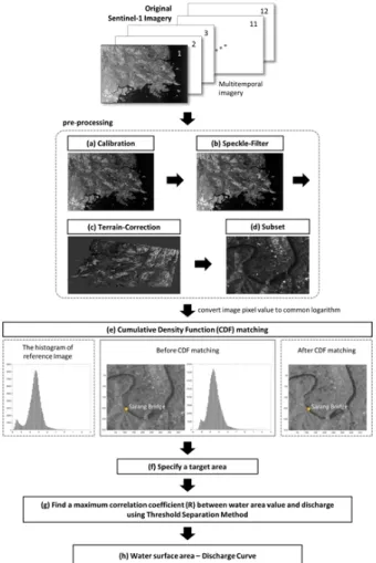
SAR 영상을 활용하여 하천의 유량을 추정하기 위해 먼저 위성 영상의 오류를 보정하는 전처리 과정을 거쳤다. 이 과정 은 ESA에서 개발한 무료 프로그램인 Sentinels Application Platform (SNAP, http://step.esa.int/main/download)을 이용 하였다. Fig. 2는 전처리 과정을 포함한 연구 과정을 보여준다.
먼저, 이미지의 픽셀값을 레이더 후방 산란 값으로 변환하 기 위하여 Calibration 과정을 거쳤다(Fig. 2(a)). 초기 이미지 픽셀값은 방사보정이 되어있지 않아 방사 측정시의 편차가 남아있다. 그러므로 이미지의 픽셀값이 실제로 레이더 후방 산란 값을 나타낼 수 있도록 방사보정 과정을 거쳐야한다 (Poenaru et al., 2015). 이 과정은 특히 본 연구와 같이 서로 다른
시간에 얻어진 이미지들을 비교할 때 필수적인 과정이다.
다음으로 산란에 의해 발생한 밝거나 어두운 점들인 Speckle 을 제거하기 위하여 Speckle filtering 과정을 거쳤다(Fig. 2 (b)). SNAP 프로그램에서는 다양한 분포 형태의 노이즈들을 처리하기 위하여 Mean, Median, Lee, Lee Sigma, Gamma- MA 등 8개의 필터를 지원한다. 본 연구에서는 노이즈를 가우 시안 분포로 가정하는 Lee Sigma 필터를 사용하여 필터링을 하였다. 이 필터는 관심 픽셀의 값을 지정된 범위 내에 있는 모든 픽셀값의 평균으로 바꿔준다(Lee, 1983; Mansourpour et al., 2011).
그리고 지형 보정(Range-Doppler terrain correction)을 통 해 이미지의 좌표체계를 WGS84 좌표계로 변환시키고 보정 하였다(Fig. 2(c)). 이를 통해 지형변화와 위성 센서의 기울기 에 의한 왜곡을 보정하여 이미지의 기하학적인 형태가 실제와 최대한 가깝도록 만들었다(Duc et al., 2017). 이후 이미지를 대상 하천 영역으로 잘라냈다(Fig. 2(d)).
2.3.2 하천 면적 추출 및 유량 추정
위성 영상은 동일한 지역을 동일한 궤도에서 촬영했더라 도 촬영 당시의 기후조건, 일조량 등에 따라 영상의 밝기와 대 비가 각기 다르다(Dellepiane and Elena, 2012). 한 관측소에 서 촬영한 여러 시기의 위성 영상에서 하천의 면적을 추출할 때, 모든 영상의 이미지의 밝기 분포를 동일하게 만들어 주기 위하여 누적 분포 함수 Cumulative Distribution Function (CDF)을 활용한 Histogram Matching 기법(Homer et al., 1997;
Helmer and Ruefenacht, 2005; Bourke, 2011; Kim and Kim, 2014)을 활용하였다(Fig. 2(e)). 이를 통해 각 관측소 내 모든 이미지의 히스토그램을 기준 이미지의 히스토그램과 일치하 게 바꿔주었다. 이때, 이미지의 픽셀값은 밝기를 나타내며 이 는 0과 1사이의 값으로 최대값과 최소값의 차이가 매우 커 log 를 취했으며, 너무 밝거나 어둡지 않고 하천의 경계가 뚜렷한 이미지를 기준 이미지로 선정하였다.
밝기 분포를 일치시킨 이미지에서 임계치 분류방식 Threshold Separation Method로 하천 영역을 추출하여 하천의 면적과 유량의 상관관계를 파악하고 관계식을 구하였다(Fig. 2(g) and Fig. 3(b)). 임계치 분류방식은 특정 임계값(threshold)을 기준으로 수체와 비수체를 분류하는 방법이다. SAR 영상에 서 수체는 후방 산란 값이 작아 주변의 비수체보다 픽셀값이 작으며 어둡게 나타나므로 임계값보다 픽셀값이 작으면 수체, 임계값보다 크면 비수체로 분류하였다(Otsu, 1979; Matgen et al., 2011; Twele, 2016). 이때, 임계치 분류방식을 이미지 내 전체 픽셀에 적용할 경우, 타 하천 및 주변 시설물, 토지이용 등의 영향을 받는다. 그러므로 관측소와 관련된 하천만을 추
Fig. 2. Schematic showing the overall methodology
출하고 타 영향을 최소화하기 위하여 특정 하천 영역을 다각 형으로 잘라 분리한 후(Fig. 3(a)의 점선), 잘라낸 다각형 내의 픽셀값들에 대하여 임계치 분류방식을 적용하였다.
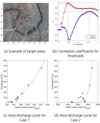
또한, 다음과 같은 과정을 반복하여 하천의 면적과 유량과 의 상관관계를 가장 잘 나타내는 하천 영역과 임계값을 산출하 였다(Fig. 3). 이 과정을 통해 보다 정확한 하천 면적과 유량의 상관관계식을 구할 수 있었다. 먼저, 특정 하천 영역을 다각형 으로 잘라 분리한 후, 수체와 비수체를 분류하는 임계값의 범 위 내에서 하나의 특정 임계값을 선택하여 12장의 사진 각각 에 대하여 수체와 비수체를 분류하였다. 이를 통해 추출된 12 개의 수체면적과 각각의 촬영 시간에 해당하는 하천 유량과의 상관계수를 도출하였다. 여기에서, 하천의 면적과 유량의 상 관관계식은 멱함수 관계를 갖는 것으로 가정하였다(Leopold and Maddock, 1953; Smith et al., 1996; Govindasamy et al., 2012; Kim and Paik, 2015; Sichangi et al., 2016). 그리고 임계 값을 바꾸며 수체와 비수체를 분류하는 과정을 반복 하면서 수체면적과 하천 유량의 상관관계가 가장 높게 도출되는 임계 값을 기록하였다. 마지막으로, 이 과정을 다양한 다각형 지역 에 대하여 시도하며 수체면적과 하천 유량의 상관관계가 가장 높게 도출되는 다각형 지역과 임계값을 선택하였다.
Fig. 4는 사랑교 지점에서 서로 다른 수체-비수체 임계값 및 다각형 지역(Case 1과 Case 2)에 대하여 변화하는 수체면적- 유량과의 상관계수를 보인다. Fig. 4(a)에 나타낸 두 가지 경우 의 다각형 지역에 대해서, 임계값에 따른 상관계수의 변화를 Fig. 4(b)에 나타냈다. 상관계수가 최대일 때의 임계값을 이용 하여 하천 면적을 추출하고 이를 통해 얻은 하천 면적과 유량 의 상관관계를 Fig. 4(c) and Fig. 4(d)에 나타냈다. Case 1이 Case 2보다 상관계수가 높게 나타났으며 따라서 그래프의 상 관관계 또한 Case 1이 뚜렷하게 나타났다. Case 2의 경우, 선 택한 다각형 지역이 강의 합류 지점을 포함하여 상관관계가 Case 1에 비하여 뚜렷하게 나타나지 않은 것으로 파악된다.
3. 결 과
3.1 유량 추정시 영향 인자
인공위성 자료는 지형 및 식생, 토지 이용 및 도로, 고층 건 물에 의한 그림자 등의 영향을 받는다(Kandus et al., 2001;
Hostache et al., 2012; Liu, 2016). 이에 의한 영향을 줄이기 위하여 본 연구에서는 Fig. 3(a)와 같이 하천 주변 영역을 분리 하여 분석하였는데, 이러한 과정은 자동화되지 않아 하천을 포함한 주변지역을 육안으로 확인하며 다각형의 모양으로 선 택해야만 한다. 이 과정에서 주의해야 할 점은 다음과 같다:
(1) 다른 하천의 영향을 받지 않도록 하천이 합류 또는 분리되 는 지점과 떨어진 영역을 선택해야 한다 (Fig. 4); (2) 댐이나 수력 발전소와 같은 하천의 자연스러운 흐름을 방해하는 시설 물이 설치되어 영향을 받는 지역과 하천 주변이 정비되어 유 량변화에 따라 하천의 면적 변화가 적은 곳을 피해야 한다; (3) 이와 반대로, 하천 내에 모래섬이 있거나 하천 주변이 유량 변
Fig. 3. Algorithm of finding an optimal target area and a maximum correlation coefficient
(a) Example of target areas (b) Correlation coefficients for thresholds
(c) Area-discharge curve for
Case 1 (d) Area-discharge curve for Case 2
Fig. 4. (a) Target areas for case 1 and case 2 at Sarang Bridge; (b)
Correlation coefficient between the water area and discharge
varying with different water extraction threshold. Two
different curves correspond to different cases of target area
(two polygons shown in Fig. 4(a)).; (c) Relationship between
the extracted water surface area and discharge based on
the target area case 1; (d) Relationship between the extracted
water surface area and discharge based on the target
area case 2
화에 민감하게 반응하는 곳을 선택하면 정확한 모형을 얻을 수 있다.
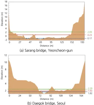
또한, 하천 단면의 측면 경사가 유량에 따른 하천 면적의 변 화에 영향을 준다. Fig. 5에 15개 관측소의 하천 단면의 평균 측면 경사와 결정 계수의 관계를 나타냈다. 유량추정모형 구 축에 실패한 안흥교는 결정 계수를 0으로 나타냈다. 이를 통해 하천 단면의 평균 측면 경사가 커질수록 유량추정모형의 결정 계수가 낮아지는 경향성을 확인할 수 있었다. 이는 측면 경사 가 완만할 경우 유량 변동에 따라 하천 폭이 민감하게 반응하 고 면적의 변화 또한 크지만, 경사가 급할 경우 유량에 따른 면적의 변화를 파악하기 어렵기 때문이다.
Fig. 6은 모형의 성능이 가장 좋았던 경우인 (a) 사랑교와 함께 사랑교와 폭은 비슷하지만 모형의 성능이 낮았던 (b) 대 곡교의 하천 단면을 보인다. 사랑교의 경우, 평균적으로 완만 한 경사를 가지고 있어 최저 수위일때와 최고 수위일 때의 폭 의 차이가 크다. 한편, 대곡교는 경사가 급하고 수위 및 유량에 따른 하천 폭의 차이가 적다. 이에 따라 사랑교는 유량추정모 형의 정확도가 높고(R2=0.99), 대곡교는 그보다 낮게 나타났 다(R2=0.5).
3.2 유량추정모형의 한계점
본 연구에서 구축한 유량추정모형은 지상 관측 자료와 인 공위성 영상 자료를 사용하여 하천의 면적과 유량의 관계식을 산출하고 이를 통해 유량을 추정하는 모형이다. 따라서 인공 위성 영상 촬영 당시의 지상 관측 자료가 필수적으로 요구된 다. 기존 지상 관측 자료가 없는 곳의 경우, 먼저 위성 영상 촬영 시간과 동일한 시간의 유량자료를 확보하여야 한다. 또한 다 양한 범위에서 유량을 정확하게 예측하기 위해서, 저유량 자
료뿐만 아니라 고유량일 때의 자료가 모두 필요하다.
지상 관측 자료의 필요성과 함께 인공위성 영상의 해상도 또한 본 모형의 한계점이다. 연구에서 사용한 Sentinel-1 위성 영상의 공간 해상도는 약 20 m이다. 분석이 불가능 했던 안흥 교의 경우, 하천 폭이 30-50 m로 인공위성의 공간 해상도에 비해 좁아 위성 영상에서 수체와 비수체를 구별할 수 없어 하 천 면적을 추출할 수 없었다. 이를 통해 폭 50 m 이하의 좁은 하천의 경우 본 연구가 제안하는 기법을 통해 하천의 면적을 정확하게 추출하기 어려우며, 이에 따라 유량에 따른 하천 면 적의 변동을 파악하기 어렵다는 점을 알 수 있다. Fig. 7에 본 연구에서 모형의 성능이 가장 좋았던 사랑교와 모형 구축에 실패한 안흥교에서 2017년 7월 13일 06시 31분(한국 시간 기 준)에 촬영한 전처리 과정을 마친 인공위성 영상을 보였다.
Fig. 5. Relationship between the average side slope and coefficient of determination for the 15 gauge stations
(a) Anheung bridge, Hoengseong-gun (b) Sarang bridge, Yeoncheon-gun Fig. 7. Sentinel-1 satellite imagery of (a) Anheung Bridge where water surface area-flow discharge relationship could not be derived and that of (b) Sarang Bridge where water surface area-flow discharge relationship could be clearly derived
(a) Sarang bridge, Yeoncheon-gun
(b) Daegok bridge, Seoul
Fig. 6. A side slope of the cross section at the Sarang bridge and the
Daegok bridge
3.3 유량추정 결과
한강 유역 내 15개 관측소에서 하천의 유량을 추정하기 위 하여 2015년 1월 1일부터 2017년 10월 31일까지의 각 관측소 별 12개의 Sentinel-1 위성 영상 자료와 관측소 유량자료를 활 용하였다. 그 결과, 강원도 횡성군에 위치한 안흥교 1개소를 제외한 14개 관측소에서 하천 면적을 입력 자료로 하는 멱함 수 형태의 유량추정모형을 구축할 수 있었다. 또한 각 관측소
별 6개의 Sentinel-1 위성 영상 자료와 관측소 유량자료를 검 증자료로 활용하였다. 각 관측소별 유량추정모형 구축시 얻 은 임계값으로 수체의 면적을 추출한 후 유량추정모형으로 추정한 유량 값과 실제 관측소 유량자료와의 비교를 통해 유 량추정모형을 검증하였다.
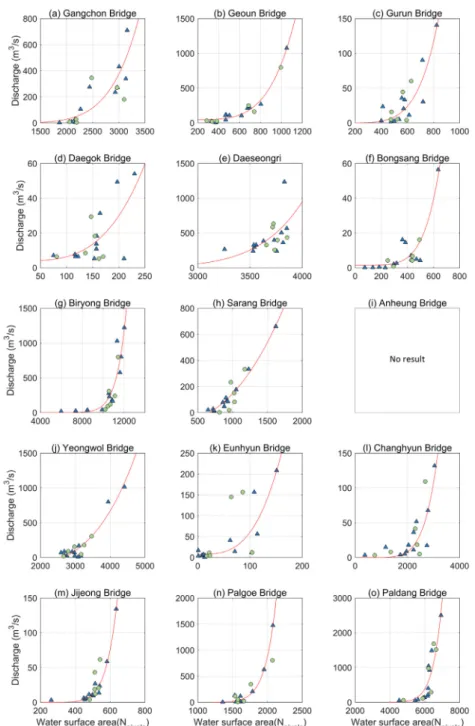
Fig. 8에 그 결과를 보였다. 그래프의 x축은 인공위성 자료 에서 추출한 수체의 면적이고 y축은 유량을 나타낸다. 실선은
Fig. 8. Relationship between the extracted water surface area (x) and the flow discharge (y) for the 15 gauge stations. The blue triangles
represent data for constructing a model, The red lines represent a discharge estimation model and the circles represent validation data
본 연구에서 구축한 멱함수형태의 유량추정모형을 나타내 며, 삼각형과 원형 표식은 유량추정모형을 구축 및 검증하는 데 사용한 자료를 각각 나타낸다. 따라서 그래프의 표식이 실 선에 가까울수록 유량추정모형의 정확도가 높으며, 검증 자 료인 원형 표식이 대부분 유량추정모형과 동일하거나 유사한 값을 나타내는 것을 확인하였다.
Table 3은 하천 면적을 이용한 유량추정모형의 모수와 결 정 계수(R2) 및 평균 제곱근 오차(Root Mean Square Error)를 나타낸다. 14개 관측소의 평균 결정 계수(R2)는 0.8로 대부분 의 관측소에서 높게 나타났다. 14개 관측소 중 결정 계수가 0.5 이하인 관측소가 두 군데 존재하였는데, 서울시 대곡교의 경 우 하천 폭이 40-60 m로 좁아 하천 면적 추출 시 정확도가 떨어 지는 것으로 판단되며, 가평군 대성리는 하천의 폭은 약 250 m 로 넓지만 하천 단면의 측면 경사가 급해 유량이 크게 변화하 여도 인공위성에 바라본 하천의 면적의 변화가 크지 않아 정 확도 높은 유량추정모형을 구축하는데 어려움이 있는 것으로 파악되었다. Fig. 9은 대성리의 하천 단면을 나타내며 최대 수 위와 최소 수위의 하천 폭 차이가 크지 않음을 알 수 있다. 이를 통해 본 연구가 제안하는 수체-유량 추정모형 구축 시 하천의 폭보다, 하천 단면의 측면 경사가 중요한 영향을 미치는 것을 파악했다.
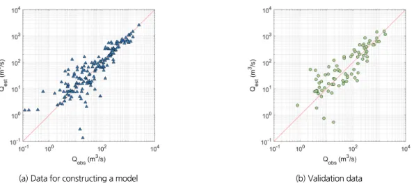
Fig. 10에 14개 관측소의 관측소 유량과 본 연구에서 구축 한 모형으로 추정한 유량의 관계를 나타냈다. Fig. 10(a)는 모
형 구축에 사용한 자료의 관측소 유량과 모형 추정 유량의 관 계도이며 Fig. 10(b)는 검증에 사용한 자료의 관측소 유량과 모형 추정 유량의 관계를 보여준다. x축은 관측소 유량을 나타 내고 y축은 모형을 통해 추정한 유량을 나타낸다. 자료의 분포 가 실선에 가까울수록 모형의 성능이 우수함을 의미하며, 모 형 구축에 사용한 자료와 검증 자료 모두 실선에 가깝게 나타 나 본 모형의 성능이 좋음을 알 수 있었다. 또한 유량 값이 클 때 더욱 실선에 가깝게 나타난 것으로 보이지만 로그 축을 사 용했으므로 절대적인 값의 차이로 볼 때, 유량 값이 작을 때에 도 모형의 성능이 우수하다고 판단된다.
따라서, 결과들을 종합적으로 볼 때, 본 연구에서 구축한 유 량추정모형의 정확도가 높은 것으로 판단된다.
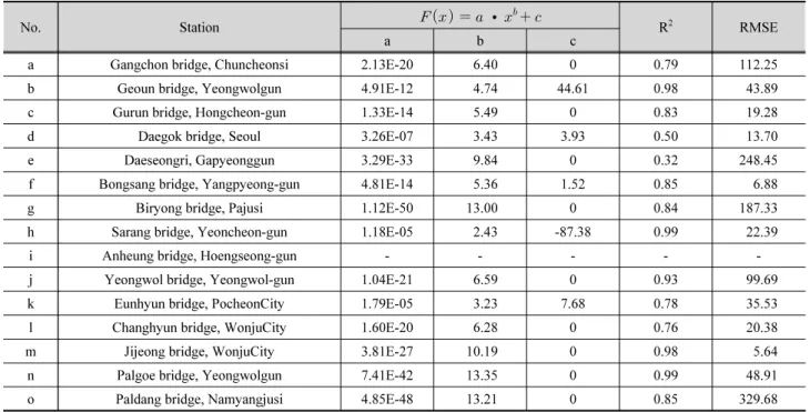
Table 3. Correlation equation in water surface area and discharge
No. Station ∙
R
2RMSE
a b c
a Gangchon bridge, Chuncheonsi 2.13E-20 6.40 0 0.79 112.25
b Geoun bridge, Yeongwolgun 4.91E-12 4.74 44.61 0.98 43.89
c Gurun bridge, Hongcheon-gun 1.33E-14 5.49 0 0.83 19.28
d Daegok bridge, Seoul 3.26E-07 3.43 3.93 0.50 13.70
e Daeseongri, Gapyeonggun 3.29E-33 9.84 0 0.32 248.45
f Bongsang bridge, Yangpyeong-gun 4.81E-14 5.36 1.52 0.85 6.88
g Biryong bridge, Pajusi 1.12E-50 13.00 0 0.84 187.33
h Sarang bridge, Yeoncheon-gun 1.18E-05 2.43 -87.38 0.99 22.39
i Anheung bridge, Hoengseong-gun - - - - -
j Yeongwol bridge, Yeongwol-gun 1.04E-21 6.59 0 0.93 99.69
k Eunhyun bridge, PocheonCity 1.79E-05 3.23 7.68 0.78 35.53
l Changhyun bridge, WonjuCity 1.60E-20 6.28 0 0.76 20.38
m Jijeong bridge, WonjuCity 3.81E-27 10.19 0 0.98 5.64
n Palgoe bridge, Yeongwolgun 7.41E-42 13.35 0 0.99 48.91
o Paldang bridge, Namyangjusi 4.85E-48 13.21 0 0.85 329.68
Fig. 9. Cross section at the Daeseongri, Gapyeonggun. The green
line represents maximum water level and the blue line
represents minimum water level
4. 결 론
본 연구에서는 기존의 관측소 유량 추정 방법의 한계를 극 복하기 위하여 인공위성을 활용한 유량추정모형을 구축하였 다. 유럽항공우주국 Sentinel-1 위성의 SAR 영상과 지상 관측 소 유량 자료를 입력 자료로 활용하여, 한강 유역 내 15개 관측 소의 하천 유량을 추정하였다. SAR 영상은 오류보정을 위한 전처리 과정과 밝기 분포를 동일하게 만들어주는 Histogram Matching 기법을 거쳤으며, 임계치 분류 방식 Threshold Separation Method 로 영상에서 하천의 면적을 추출하였다.
추출한 면적과 유량의 관계식을 도출하여 유량추정모형을 구축한 결과, 1개소를 제외한 14개 관측소에서 하천 면적을 입력 자료로 하는 멱함수 형태의 유량추정모형을 구축할 수 있었다. 14개 관측소의 평균 결정 계수(R2)는 0.8로 대부분의 관측소에서 높게 나타났으며 다양한 크기의 하천에서 정확도 높은 결과를 얻을 수 있었다.
모형 구축에 실패한 안흥교의 경우, 하천 폭이 좁아 위성 영 상에서 수체와 비수체를 구별하기 어려워 면적을 추출할 수 없었다. 이를 통해 위성의 공간 해상도(약 20 m)의 영향으로 인해, 폭 50 m 이하의 좁은 하천 및 경사가 급한 하천의 경우 모형 구축이 어렵다는 점을 파악할 수 있었다. 그 밖에도 모형 구축 시 관측소 유량 자료가 필요하고 하천 주변의 지형 및 시 설물 등의 영향을 받는 한계가 있어 경사가 완만하고 유량 변 동에 따라 하천 폭이 민감한 망상 하천과 같은 하천에 활용 범 위가 한정된다는 단점이 있었다. 하지만, 이러한 한계점들은 위성 영상의 공간 및 시간 해상도의 성능이 향상됨에 따라 개 선될 것으로 기대된다.
본 연구의 결과가 유량관측소가 설치되지 않은 중소규모
의 다양한 하천에서 유량자료를 구축하는데 기여할 수 있기를 기대한다.
감사의 글
본 연구는 환경부의 물관리연구사업에서 지원받았습니다 (18AWMP-B079625-05).
References