Spatial Distribution Pattern of the Populations of Cephalanthera erecta at Mt.
Ahop in Busan
Man Kyu Huh*
Department of Molecular Biology, Dong–eui University, Busan 47340, Korea Received April 11, 2016 /Revised July 4, 2016 /Accepted July 6, 2016
Cephalanthera erecta (Thunb. ex, Murray) is an herbaceous and a member of the genus Cephalanthera in the family Orchidaceae. The species is an herbaceous and has reputed Chinese medicinal value. It has been investigated the population density and spatial distribution of this species at Mt. Ahop in Korea during 2015. The spatial pattern of C. erecta was analyzed according to several patchiness in- dexes, population uniformity or aggregation under different sizes of plots by dispersion indices, and spatial autocorrelation. The mean crowding (M*) and patchiness index (PAI) showed positive values except one small plot (2 m × 2 m). Most natural individuals of C. erecta for plots were not uniformly distributed in the forest community. The small plots (2 m × 2 m, to 8 m × 16 m) of C. erecta were uniformly distributed in the forest community and large plots (16 m × 16 m and 16 m × 32 m) were aggregately distributed. Significant aggregations by Moran's I of C. erecta were partially observed within IV classes (12 m). Dissimilarity among pairs of individuals could found by more than 18.0 m.
In conclusion, the geographic distribution of C. erecta is not even with varying degrees of size of plots and human activities give rise to density effects in the plots at Mt. Ahop in Korea.
Key words : Cephalanthera erecta, Mt. Ahop, Moran's I, patchiness indexes, spatial distribution
*Corresponding author
Tel : +82-51-890-1529, Fax : +82-505-182-6870
*E-mail : [email protected]
This is an Open-Access article distributed under the terms of the Creative Commons Attribution Non-Commercial License (http://creativecommons.org/licenses/by-nc/3.0) which permits unrestricted non-commercial use, distribution, and reproduction in any medium, provided the original work is properly cited.
Journal of Life Science 2016 Vol. 26. No. 8. 881~886 DOI : http://dx.doi.org/10.5352/JLS.2016.26.8.881
Introduction
Plant survival and growth depend on local environments within a habitat [7, 11]. Spatial pattern (distribution of in- dividuals in space) is an important characteristic of pop- ulations of sedentary organisms. Spatial configuration of suitable environments for plants is often patchily structured at various sizes within the habitat, like islands in a sea [22].
The spatial distribution pattern of plant populations exhibits scale dependence, e.g. a species may show an aggregated distribution at one spatial scale and may change to a ran- dom or uniform distribution at a different scale [12].
Botanists, ecologists, and population genetic researches have been interested in studying plant distribution patterns as they provide insight into the processes that facilitate diversi- fication and speciation in plants and the factors that lead to reproductive isolation between closely related plant pop- ulations [25]. Many models of development of spatial pat-
terns showed a trend of making regular distribution, when they were of nearly the same age and made densely closed canopy. Under their modeling assumptions they have shown that both random and aggregated spatial patterns of natural even-aged forest stands over time are preserved over time and a regular (lattice) spatial pattern tends to change into a random spatial pattern [13].
Analysis of the spatial distribution pattern of a plant pop- ulation is helpful to determine the population’s ecological preferences, biological characteristics and relationships with environmental factors [26]. Therefore, the analysis of the spatial distribution pattern of plant populations has always been a major focus for ecological research [2, 10].
Many ecologists have adopted several different major schools of spatial analysis from other disciplines [16]. The first of these comes from geography, and its methods in- clude the use of statistics (e.g., Moran’s I) to measure spatial autocorrelation [19]. It measures the extent to which the occurrence of an event in a real unit constrains, or makes more probable, the occurrence of an event in a neighboring areal unit.
Cephalanthera erecta (Thunb. ex, Murray) is an herbaceous
and a member of the genus Cephalanthera in the family
Orchidaceae. C. erecta is found in the far eastern Russia,
Korea, Northern China, eastern Himalayas, Bhutan and
Japan in open forests and thicket margins at elevations of 500 to 2,300 m. Several white flowers were occurred in May and June.
In this report, the several statistical tools of percentage distribution and population structure of the geographical areas are used to study the spatial distribution of C. erecta in Busan. Mt. Ahop locate in south of the Korean. A sample of a large (more than 330 individuals) natural population of C. erecta collected and was used in this study. It is ex- pected to provide useful experimental conditions because of the large undisturbed and isolated site.
The purpose of this paper was to describe a statistical analysis for detecting a species association, which is valid even when the assumption of within- species spatial ran- domness is violated. The purpose of this study is addressed:
is there a spatial structure within populations of C. erecta?
Materials and Methods Study area
This study was carried out on the populations of C. erecta, located at Mt. Ahop (346.5 m) (35°16′N/129°11′E) in Busan-ci (Korea). It has a temperate climate with a little hot and long summer. In this region the mean annual tem- perature is 14.7℃ with the maximum temperature being 29.4℃ in August and the minimum -0.6℃ in January. Mean annual precipitation is about 1519.1 mm with most rain fall- ing period between June and August.
Sampling procedure
Many quadrats at Mt. Ahop were randomly chosen for each combination of site x habitat, so that, overall, 90 quad- rats were sampled for the complete experiment.
Spatial ecologists use artificial sampling units (so-called quadrats) to determine abundance or density of species. The number of events per unit area are counted and divided by area of each square to get a measure of the intensity of each quadrat. I randomly located quadrates in each plot which I established populations. The quadrat sizes were 2 m × 2 m, 2 m × 4 m, 4 m × 4 m, 4 m × 8 m, 8 m × 8 m, 8 m × 16 m, 16 m × 16 m, and 16 m × 32 m. I mapped all plants to estimate C. erecta density per plot.
Index calculation and data analysis
The spatial pattern of C. erecta was analyzed according to the Neatest Neighbor Rule [3, 5] with Microsoft Excel
2014.
Average viewing distance (r
A) was calculated as follows:
Where r
iis the distance from the individual to its nearest neighbor. N is the total number of individuals within the quadrat.
The expectation value of mean distance of individuals within a quadrat (r
B) was calculated as follows:
Where D is population density and D is the number of individuals per plot size.
R = r
A/ r
BWhen R > 1, it is a uniform distribution, R = 1, it is a random distribution, R < 1, it is an aggregated distribution.
The significance index of the deviation of R that departs from the number of “1” is calculated from the following formula [15].
When C
R> 1.96, the level of the significance index of the deviation of R is 5%, and When C
R> 2.58, the level is 1%.
Many spatial dispersal parameters were calculated the degree of population aggregation under different sizes of plots by dispersion indices: index of clumping or the index of dispersion (C), aggregation index (CI), mean crowding (M*), patchiness index (PAI), negative binominal dis- tribution index K, Ca indicators (Ca is the name of one in- dex) [16] and Morisita index (IM) were calculated with Microsoft Excel 2014. The formulae are as follows:
Index of dispersion:
Aggregation index
Mean crowding = m + CI = m + C-1 - 1
Patchiness index
Aggregation intensity
Ca indicators
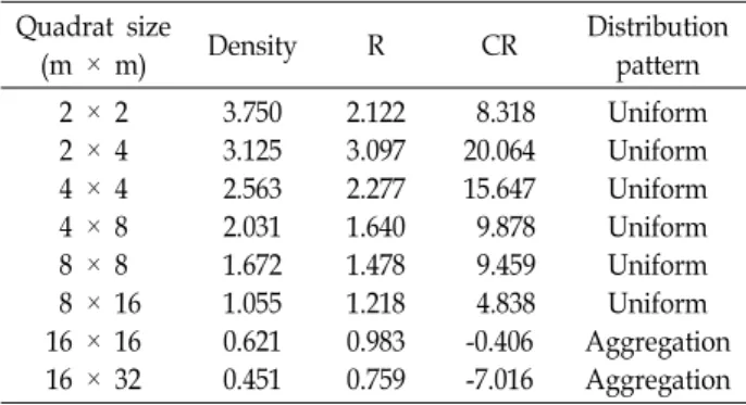
Table 1. Spatial patterns of Cephalanthera erecta individuals at different sampling quadrat sizes in Mt. Ahop Quadrat size
(m × m) Density R CR Distribution
pattern 2 × 2
2 × 4 4 × 4 4 × 8 8 × 8 8 × 16 16 × 16 16 × 32
3.750 3.125 2.563 2.031 1.672 1.055 0.621 0.451
2.122 3.097 2.277 1.640 1.478 1.218 0.983 0.759
8.318 20.064 15.647 9.878 9.459 4.838 -0.406 -7.016
Uniform Uniform Uniform Uniform Uniform Uniform Aggregation Aggregation
IM =
Where S
2is variance and m is mean density of C. erecta.
When C, M*, PAI > 1, it means aggregately distributed, when C, M*, PAI < 1, it means uniformly distributed, when CI, PA, Ca > 0, it means aggregately distributed, and when CI, PA, Ca < 0 it means uniformly distributed.
The mean aggregation number to find the reason for the aggregation of C. erecta was calculated [1].
Where r is the value of chi-square when 2k is the degree of freedom and k is the aggregation intensity.
Green index (GI) is a modification of the index of cluster size that is independent of n [9].
Spatial structure
When a plant population or community is sampled, the samples have a spatial relationship with each other. To a certain extent, samples that are close to each other are more likely to be similar. Numerical simulations of previous anal- yses were performed to investigate the significant differ- ences at various distance scales, i.e., 1.0 m, 1.5 m, 2.0 m, and so on. However, no significant population structure was found within the 3.0 m distance classes by means of Moran's I, and a significant population structure was re- vealed beyond 3.0 m. Thus, the distance classes are 0-3.0 m (class I), 3.0-6.0 m (class II), 6.0-9.0 m (class III), 9.0-12.0 m (class IV), 12.0-15.0 m (class V), 15.0-18.0 m (class VI), 18.0-21.0 m (class VII), 21.0-24.0 m (class VIII), 24.0-27.0 m (class IX), and 27.0-30.0 m (class IX).
The spatial structure was quantified by Moran's I, a co- efficient of spatial autocorrelation (SA) [19]. As applied in this study, Moran's I quantifies the similarity of pairs of spatially adjacent individuals relative to the population sample as a whole. The value of I ranges between +1 (completely positive autocorrelation, i.e., paired individuals have identical values) and -1 (completely negative auto- correlation). Each plant was assigned a value depending on the presence or absence of a specific individual. If the ith plant was a homozygote for the individual of interest, the assigned pi value was 1, while if the individual was absent, the value 0 was assigned [20].
Pairs of sampled individuals were classified according to the Euclidian distance, dij, so that class k included dij satisfying k - 1 < dij < k + 1, where k ranges from 1 to 10. The interval for each distance class was 3.0 m. Moran's
I statistic for class k was calculated as follows:
I (k) = n∑i∑j(i≠j)WijZiZj/S∑Zi
2where Zi is pi - p (p is the average of pi); Wij is 1 if the distance between the ith and jth plants is classified into class k; otherwise, Wij is 0; n is the number of all samples and S is the sum of Wij {∑i∑j(i ≠j)Wij} in class k. Under the randomization hypothesis, I (k) has the expected value u1 = -1/(n - 1) for all k. Its variance, u2, has been given, for example, in Sokal and Oden [19]. Thus, if an individual is randomly distributed for class k, the normalized I (k) for the standard normal deviation (SND) for the plant geno- type, g (k) = {I (k) - u1}/u2
1/2, asymptotically has a standard normal distribution [4]. Hence, SND g(k) values exceeding 1.96, 2.58, and 3.27 are significant at the probability levels of 0.05, 0.01, and 0.001, respectively.
Results The spatial pattern of individuals
Population densities (D) varied from 0.451 to 3.750, with a mean of 1.909 (Table 1). The values (R) of spatial distance (the rate of observed distance-to-expected distance) among the nearest individuals were higher than 1 and the sig- nificant index of CR was > 2.58. If by this parameter, the small plots (2 m × 2 m, 2 m × 4 m, 4 m × 4 m, 4 m × 8 m, 8 m x 8 m, and 8 m x 16 m) of C. erecta were uniformly distributed in the forest community (Table 1). However, C.
erecta at Mt. Ahop were aggregately distributed in two large plots (16 m × 16 m and 16 m × 32 m).
The degree of population aggregation
The values dispersion index (C) at Mt. Ahop were lower
at six plots (2 m × 2 m, 2 m × 4 m, 4 m × 4 m, 4 m × 8
m, 8 m × 8 m, and 8 m × 16 m) than 1 except two large
Fig. 1. The mean aggregation number to find the reason for the aggregation of Cephalanthera erecta.
Table 2. Changes in gathering strength of Cephalanthera erecta at different sampling quadrat sizes Quadrat size
(m × m)
No.
Quadrat
Aggregation indices
C CI M* PAI PI Ca IM
2 × 2 2 × 4 4 × 4 4 × 8 8 × 8 8 × 16 16 × 16 16 × 32
17 15 10 8 5 3 2 1
0.429 0.783 0.791 0.825 0.843 0.894 1.006 1.001
-0.575 -0.217 -0.209 -0.175 -0.157 -0.106 0.006 0.001
-0.027 0.659 0.503 0.349 0.414 0.487 0.626 0.593
-0.050 0.753 0.706 0.665 0.725 0.821 1.010 1.002
-0.953 -4.037 -3.408 - 2.989 -3.636 -5.594 99.789 456.625
-1.050 -0.248 -0.294 -0.335 -0.275 -0.179 0.010 0.002
-0.057 0.788 0.732 0.673 0.737 0.831 1.020 1.010
Fig. 2. The curves of patchiness in two areas of Cephalanthera erecta using values of Green index.
plots (Table 2). Thus these aggregation indices (CI) were negative at Mt. Ahop, which indicate a uniform distribution.
Two large plots (16 m × 16 m and 16 m × 32 m) were positive. The mean crowding (M*) and patchiness index (PAI) showed positive values except one small plot (2 m
× 2 m). The three indices C, M*, PAI were <1 and their values of PI and Ca except two plots were also shown small- er than zero, thus it means uniform distributed. In C. erecta, the two indices, C, PAI were >1 and their values of PI and Ca except four small plots were also shown greater than zero, thus it means aggregately distributed. Thus, most in- dividuals of C. erecta at Mt. Ahop were clustered and the distribution pattern of the C. erecta was quadrat-sampling dependent. The values of δ were varied from 0.012 for 8 m × 16 m to 1.105 for 2 m × 2 m (Fig. 1).
Morisita index (IM) is related to the patchiness index (PAI) and showed an overly steep slope at the plot 16 m
× 16 m in Mt. Ahop. When the area was smaller than 16 m × 16 m, the degree of aggregation increased significantly with increasing quadrat sizes, while the patchiness indices did not change from the plot 8 m × 16 m to 16 m × 32 m.
Green index varied between -0.0008 to 0.0005 (Fig. 2).
Analysis of spatial autocorrelation
The spatial autocoefficient, Moran's I is presented in
Table 3. Separate counts for each type of joined individuals and for each distance class of separation were tested for significant deviation from random expectations by calculat- ing the SND. Moran's I of C. erecta significantly differed from the expected value in 7 of 10 cases (70%). Three of these values (30.0%) were negative, indicating a partial dis- similarity among pairs of individuals in the VIII distance classes (24 m). Four of the significant values (40.0%) were positive, indicating similarity among individuals in the first 4 distance classes (I~IV), i.e., pairs of individuals can sepa- rate by more than 15.0 m. Namely significant aggregations were partially observed within IV classes. As a matter of course, the negative SND values at classes VIII, IX and X.
Thus, dissimilarity among pairs of individuals could found by more than 24.0 m.
The comparison of Moran’s I values to a logistic re- gression indicated that a highly significant percentage of individual dispersion in C. erecta populations at Mt. Ahop could be explained by isolation by distance.
Discussion
Aggregated spatial patterns with even-aged forest stands
over time are preserved over time and a regular (lattice)
spatial pattern tends to change into a random spatial pattern
Table 3. Spatial autocorrelation coefficients (Moran's I) among plots of Cephalanthera erecta for ten distance classes
I II III IV V VI VII VIII IX X
0.632*** 0.539*** 0.490*** 0.326** 0.079 -0.013 -0.055 -0.218* -0.365** -0.707***
*: p<0.05, **: p<0.01, ***: p<0.001.
[13]. These results are given for a single generation of spe- cies and no new individuals are permitted to arise during the time of development. As a homogeneous area is consid- ered, Mt. Ahop is as a relatively homogeneous area that differs from its surroundings. There is, however, a lot of field data indicating that even-aged population of trees, shrubs and herbs tend to decrease the intensity of ag- gregation in the course of self-thinning, being initially dis- tributed in clumps [24] or tend to nearly regular distribution [17, 18].
When R = 1, it is a random distribution; R < 1, it is an aggregation; R > 1, it is a uniform distribution [15].
According to this rule, individuals within short distance plots of C. erecta at Mt. Ahop are uniform distribution (Table 1). According to dispersion indices of Llord [16], when C, M*, PAI were > 1, it means aggregately distributed, when C, M*, PAI were < 1, it means uniformly distributed. In addition to, when CI, PI, Ca were > 0, it means aggregately distributed, when CI, PI, Ca were < 0, it means uniformly distributed. The small plots (2 m × 2 m, 2 m × 4 m, 4 m
× 4 m, 4 m × 8 m, 8 m × 8 m, and 8 m × 16 m) of C. erecta are not aggregately distributed (Table 2) and consistent with the Neatest Neighbor Rule [3, 15]. In only 2 large plots (16 m × 16 m and 16 m × 32 m), the three indices, C, M*, PAI were >1, and the three indices, CI, PI, Ca were > 0, thus it means aggregately distributed. To find the reason for the aggregation at larger plots, the parameter δ was calculated. When δ > 2, the aggregation was mainly caused by both species characteristics and environmental factors [15]. When δ < 2, the aggregation was mainly caused by environmental factors. The values of δ were varied from 0.012 for 8 m × 16 m to 1.105 for 2 m × 2 m. Thus, ag- gregation of C. erecta populations at Mt. Ahop is mainly caused by the environmental factors. All plots had low δ < 2. I recognized that the important environmental factors might be considered competition, growth rate, little decom- position, light, and below-ground resources. The character- istics of the C. erecta concerned included primarily their life history, artificial disturbance, and population density. Life history theory seeks to understand the variation in traits such as growth rate, number and size of offspring and life
span observed in nature, and to explain them as evolu- tionary adaptations to environmental conditions [21].
One result of spatial autocorrelation is that statistical tests performed give more apparently significant results than the data actually justify because the number of truly in- dependent observations is smaller than the number used in the test [14, 23]. A significant positive value of Moran's I indicated that pairs of individuals separated by distances that fell within distance class IV had similar individuals, whereas a significant negative value indicated that they had dissimilar individuals (Table 3). The overall significance of individual correlograms was tested using Bonferroni's criteria. The results revealed that patchiness similarity was shared among individuals within up to a scale of a 12.0 m~15.0 m distance. Thus it was looked for the presence of dispersion correlations between neighbors at this scale.
In many real populations, there may not be any obvious individual populations or substructure at all, and the pop- ulations are continuous. The results from this study are con- sistent with the supposition that a plant population is sub- divided into local demes, or neighborhoods of related in- dividuals [5, 8]. Spatially distributed genetic populations that compete locally for resources and mate only with suffi- ciently close neighbors, may give rise to spontaneous pat- tern formation [6].
References
1. Arbous, A. G. and Kerrich, J. E. 1951. Accident statistics and the concept of accident proneness. Biometrics 7, 340-342.
2. Baskent, E. Z. and Keles, S. 2005. Spatial forest planning:
a review. Ecolo. Modell. 188, 145-173.
3. Clark, P. J. and Evans, F. C. 1954. Distance to nearest neigh- bor as a measure of spatial relationships in populations.
Ecology 35, 445-453.
4. Cliff, A. D. and Ord, J. K. 1971. Spatial autocorrelation. Pion, London.
5. Ehrlich, P. R. and Raven, P. H. 1969. Differentiation of populations. Science 165, 1228-1232.
6. Epperson, B. K., Chung, M. G. and Telewski, F. W. 2003.
Spatial pattern variation in a contact zone of Pinus ponderosa and P. arizonica (Pinaceae). Am. J. Bot. 90, 25-31.
7. Farley, R. A. and Fitter, A. H. 1999. Temporal and spatial variation in soil resources in a deciduous woodland. J. Ecol.
초록:부산시 아홉산의 은난초 집단의 공간적 분포 양상 허만규*
(동의대학교 분자생물학과)
은난초(Cephalanthera erecta)는 난초과 은대난초속 초본이며 약용으로 쓰인다. 부산광역시 기장군 아홉산에서 은 난초 식물 집단에 대해 개체군의 밀도와 공간분석을 실시하였다. 은난초의 공간적 분석은 여러 공간 분석 패치 척도를 사용하여 집단의 균질한 분포와 응집이 플롯의 크기에 따라 차이가 발생하는지 조사하였으며, 플롯의 크 기에 따른 공관적 상관 분석을 실시하였다. 평균 운집 정도(M*)와 패치 지수(PAI)는 가장 작은 플롯(2 m × 2 m)을 제외하고는 양의 값을 나타내었다. 많은 플롯에서 은난초의 개체들은 숲 군집 내 일정하게 분포하지 않았다. 작은 플롯(2 m × 2 m, to 8 m × 16 m) 내 은난초 군락은 숲 군집에서 일정하게 분포하고 있었지만, 큰 플롯(16 m ×
16 m, 16 m × 32 m)에서는 은난초 군락에서 개체들의 응집이 발생하고 있었다. 공간적 상관관계 분석을 위해 Moran's I 척도를 이용한 결과 개체들의 응집은 등급 IV (12 m) 내에서 일어났다. 은난초 개체들은 18.0 m 이상 거리가 이격되면 이질성이 발생하였다. 결론적으로 한국 내 아홉산 집단에서 은난초의 지리적 분포는 플롯의 크 기에 따라 변하며, 패치(patchy)구조를 보이며 패치의 크기는 인간의 활동에 의해서 밀도 효과를 유발한 것으로 판단되었다.
87, 688-696.
8. Garnier, L. K. M., Durand, J. and Dajoz, I. 2002. Limited seed dispersal and microspatial population structure of an agamospermous grass of West African savannahs. Hypar- rhenia diplandra (Poaceae). Am. J. Bot. 89, 1785-1791.
9. Green, R. H. 1966. Measurement of non-randomness in spa- tial distributions. Res. Pop. Ecol. 8, 1-7.
10. Haase, P. 1995. Spatial pattern analysis in ecology based on Ripley’s K-function: introduction and methods of edge correction. J. Veg. Sci. 6, 575-582.
11. Huh, M. K. 2015. Spatial distribution pattern of the pop- ulations of Carex siderosticta at Mt. Geumjeong and Mt.
Ahop. J. Life Sci. 25, 369-375.
12. Kang, M. K and Huh, M. K. 2014. Spatial distribution pat- tern of the populations of Camellia japonica in Busan. J. Life Sci. 24, 813-819.
13. Leps, J. and Kindlmann, P. 1987. Models of the develop- ment of spatial pattern of an even-aged plant population over time. Ecol. Modell. 39, 45-57.
14. Legendre, P. 1993. Spatial autocorrelation: trouble or new paradigm? Ecology 74, 1659-1673.
15. Lian, X., Jiang, Z., Ping, X., Tang, S., Bi, J. and Li, C. 2012.
Spatial distribution pattern of the steppe toad-headed lizard (Phrynocephalus frontalis) and its influencing factors. Asian Herpet. Res. 3, 46-51.
16. Lloyd, M. 1967. Mean crowding. J. Ani. Ecol. 36, 1-30.
17. Phillips, D. L. and MacMahon, J. A. 1981. Competition and spacing patterns in desert shrubs. J. Ecol. 69, 97-115.
18. Prach, K. 1981. Selected ecological characteristics of shrubby
successional stages on abandoned fields in the Bohemian Karst. Preslia 53, 159-169
19. Sokal, R. R. and Oden, N. L. 1978a. Spatial autocorrelation in biology 1. Methodology. Biol. J. Lin. Soc. 10, 199-228.
20. Sokal, R. R. and Oden, N. L. 1978b. Spatial autocorrelation in biology 2. Some biological implications and four applica- tions of evolutionary and ecological interest. Biol. J. Lin.
Soc. 10, 229-249.
21. Souza, A. F. and Martins, F. R. 2004. Microsite special- ization and spatial distribution of Geonoma brevispatha, a clo- nal palm in south-eastern Brazil. Ecol. Res. 19, 521-532.
22. Suzuki, R. O., Sujuki, J. I. and Kachi, N. 2005. Change in spatial distribution patterns of a biennial plant between growth stages and generations in a patchy habitat. Ann.
Bot. 96, 1009-1017.
23. Thomson, J. D., Weiblen, G., Thomson, B. A., Alfaro, S.
and Legendre, P. 1996. Untangling multiple factors in spa- tial distribution: lilies, gophers, and rocks. Ecology 77, 1698- 1715.
24. Williams, D. G., Anderson, D. J. and Slater, K. R. 1978.
The influence of sheep on pattern and process in Atriplex oesicaria populations from the Riverine Plain of New South Wales. Aust. J. Bot. 26, 381-392.
25. Woodward, F. I. 1987. Climate and plant distribution.
Cambridge Univ. Press, Cambridge, UK.
26. Zhang, Y. T., Li, J. M., Chang, S. L., Li, X. and Lu, J. J.
2012. Spatial distribution pattern of Picea schrenkiana pop- ulation in the Middle Tianshan Mountains and the relation- ship with topographic attributes. J. Arid Land 4, 457-468.