Spatial Distribution Patterns of Oplismenus undulatifolius var. undulatifolius on Mt. Hanwoo in Korea

Spatial Distribution Patterns of Oplismenus undulatifolius var. undulatifolius on Mt. Hanwoo in Korea

Man Kyu Huh*

Division of Applied Bioengineering, Dong-eui University, Busan 47340, Korea

Received July 4, 2018 /Revised November 7, 2018 /Accepted November 17, 2018

The patchiness of local environments within a habitat is assumed to be a primary factor affecting the spatial patterns of plants. In this study, a randomization procedure was developed to test the null hypothesis that only spatial association with patches determines the spatial patterns of plants.

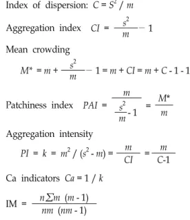
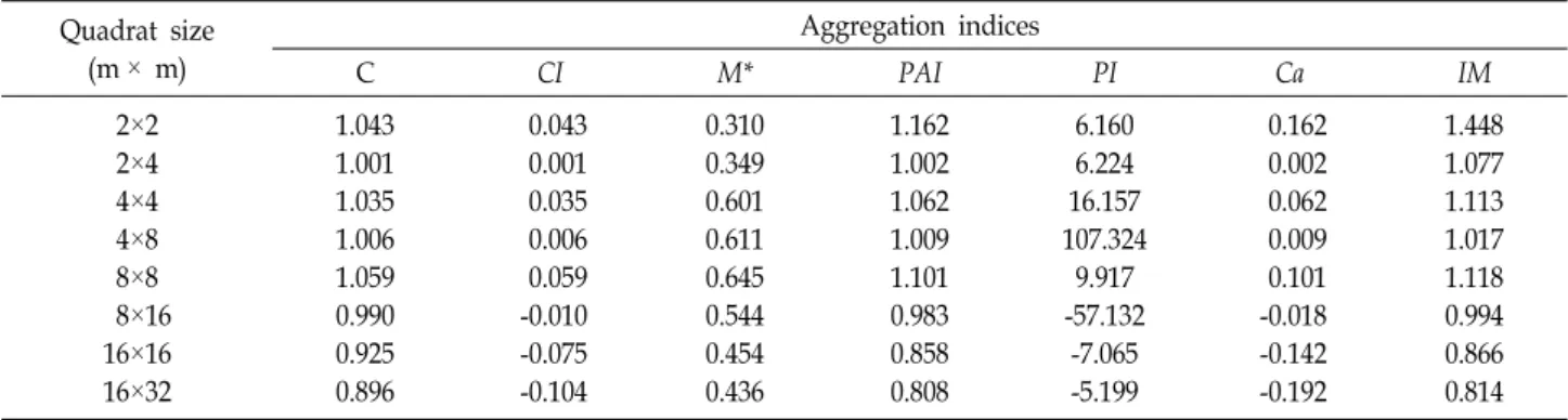
Oplismenus undulatifolius (Ard.) P. Beauv. var. undulatifolius is an herbaceous plant and a member of the genus Oplismenus in the family Poaceae. Oplismenus hirtellus subsp. undulatifolius occurs in temper- ate, subtropical, and tropical areas of the world. The spatial pattern of O. undulatifolius var. un- dulatifolius was analyzed using dispersion indices in different sizes of plots according to several patch- iness indexes, population uniformity, or aggregation . Population densities (D) at Mt. Hanwoo varied from 0.453 to 4.375, with a mean of 2.387. The small and mid-sized plots (2 m × 2 m, 2 m × 4 m, 4 m × 4 m, 4 m × 8 m, and 8 m × 8 m) of O. undulatifolius var. undulatifolius were aggregated in the forest community. However, O. undulatifolius var. undulatifolius was uniformly distributed in three large plots (8 m × 16 m, 16 m × 16 m, and 16 m × 32 m). The greatest mean crowding (M*) and patchiness index (PAI) showed positive values. Aggregation is mainly caused by environmental factors. Many plants on Mt. Hanwoo are being disturbed by climbers, which is preventing these plants from inhabiting their realized niches on Mt. Hanwoo.

Key words : Mt. Hanwoo, Oplismenus undulatifolius var. undulatifolius, patchiness index, spatial distribution

*Corresponding author

*Tel : +82-51-890-1529, Fax : +82-505-182-6870

*E-mail : [email protected]

This is an Open-Access article distributed under the terms of the Creative Commons Attribution Non-Commercial License (http://creativecommons.org/licenses/by-nc/3.0) which permits unrestricted non-commercial use, distribution, and reproduction in any medium, provided the original work is properly cited.

Journal of Life Science

Introduction

The spatial distribution of vegetation is commonly used by plant ecologists to determine relationships among plants and to better understand plant community dynamics [5].

Spatial statistics provides the quantitative description of nat- ural variables distributed in space and time and now it is the most rapidly growing field in ecology [13]. Spatial anal- yses are commonly used in many disciplines, such as plant and animal ecology, geography, archeology or mining engineering. It has also found applications in forestry and forest science. Studying the spatial distribution of species according to their niche breadth would normally be ad- dressed by studying spatial organization using, e.g. multi- variate analysis, and trying to interpret observed associa- tions according to the distance from an individual to its nearest neighbor, irrespective of direction.

For any species, factors limiting its distribution include a combination of biotic and abiotic factors that may operate at different spatial and temporal scales [14].

Aggregated patterns of plants are often observed as spa- tial structures in a local population especially in a patchy habitat, and these are scale-dependent [17]. Aggregated pat- terns at the spatial scale corresponding to the size of patches would be the result of spatial variation in mortality and establishment of plants caused by the patchiness of the envi- ronment [9].

Structures and dynamics of a local population in a patchy habitat also depend on the structure of the habitat, which is called patch dynamics [8, 19], although it is usually ap- plied to the large-scale dynamics of a regional population at landscape level [17]. However, spatially distribution de- termine at a local population in Korea has rarely been studied.

Oplismenus undulatifolius (Ard.) P. Beauv. var. undulatifolius

is a species of perennial grass from the Poaceae family that

is native to South Asia, East Asia, Southeast Asia, Australia,

and Southern Africa. Thus the species can be found in tem-

perate, subtropical, and tropical areas of the world such

as Pakistan (Punjab and Kashmir), China, Japan, Korea,

India, Australia, South Africa, Madagascar [15].

O. undulatifolius var. undulatifolius spreads rapidly through wooded natural areas, crowding out native herbaceous plants and preventing regeneration of native hardwood tree species. It forms dense carpets in the forest understory, at times creating a new layer of plant vegetation in habitats [18].

The aims of this study were to: (i) estimate plant density and population size of O. undulatifolius var. undulatifolius at Mt. Hanwoo in Korea, (ii) explore the spatial patterns of particular plot size variables and evaluate how these might be associated with the abundance and distribution of this species.

Materials and Methods Study area

This study was carried out on the populations of O. un- dulatifolius var. undulatifolius, located at Mt. Hanwoo (835 m) (35°398‘251’‘N/128°188’601‘’E) in Uiryeong-gun, Gyeong- sangnam-do Province in Korea. The mountain is alpine mountain trail well maintained up to the mountain top.

Especially, the place where this plant grows is the area where the mountain trail of Mt. Hanwoo is combined with the mountain trail of Mt. Jagul (897 m). The forest site com- prised of rich vegetation which had not been disturbed for more than sixty years while the farming-land had almost no vegetation due to frequent human activities and interfer- ence. The elevation of community of O. undulatifolius var.

undulatifolius ranges from 400 to 500 m. The site is charac- terized by a temperate climate with a little hot and long summer. The mean annual temperature is 13.0℃ with the maximum temperature being 25.4℃ in August and the min- imum -0.5℃ in January. The mean annual precipitation ranges from 15.2 (December) to 294.5 mm (August) with 1275.6 mm. The rain is concentrated in rain falling period between June and August.

Sampling procedure

Spatial ecologists use artificial sampling units (so-called quadrats) to determine abundance or density of species.

Many quadrats at Mt. Hanwoo were randomly chosen for each combination of site x habitat, so that, overall, 46 quad- rats were sampled for the complete experiment. The quadrat sizes were 2 m × 2 m, 2 m × 4 m, 4 m × 4 m, 4 m × 8 m, 8 m × 8 m, 8 m × 16 m, 16 m × 16 m, and 16 m × 32 m.

Index calculation and data analysis

The spatial pattern of O. undulatifolius var. undulatifolius was analyzed according to the Neatest Neighbor Rule [3, 11] with Microsoft Excel 2016. The distance from an in- dividual to its nearest neighbor, irrespective of direction, provides the basis for this measuring of spacing [3].

The mean observed distance (r

) was calculated as fol- lows:

r

= ∑

ri / N (i = 1, 2, 3 ... N)

Where r

is the distance from the individual to its nearest neighbor. N is the total number of individuals within the quadrat.

If this population were distributed at random, the expect- ation value of mean distance of individuals within a quadrat (r

) was calculated as follows:

⎯ r

= 1/2√D

Where D is population density and D is the number of individuals per plot size. The ratio R can be used as a meas- ure of the degree to which the observed distribution ap- proaches or departs from random expectation.

R = r

/ r

When R > 1, it is a uniform distribution and R < 1, it is an aggregated distribution. In a random distribution, R

= 1 and under conditions of maximum aggregation, R = 0.

If the value of R is not randomly distributed, the sig- nificance of the deviation is calculated from the following formula [3].

C

= r

－ r

δ

⎯⎯

δ

= 0.26136 / √ND

When C

> 1.96, the level of the significance index of the deviation of R is 5%, and When C

> 2.58, the level is 1%.

One test for spatial pattern and associated index of dis- persion that can be used on random-point-to-nearest-organ- ism distances was suggested by Eberhardt [4] and analyzed further by Hines and Hines [7]: I

= (s/m)

+ 1

Where I

= Eberhardt’s index of dispersion for point-to-or- ganism distances, s = observed standard deviation of dis- tances, m = mean of point-to-organism distances.

Many spatial dispersal parameters were calculated the

degree of population aggregation under different sizes of

plots by dispersion indices: index of clumping or the index

Table 1. Spatial patterns of Oplismenus undulatifolius var. undulatifolius individuals at different sampling quadrat sizes in Mt. Hanwoo

Quadrat size (m × m) No. Quadrat Density R CR I

Distribution pattern

2×2 2×4 4×4 4×8 8×8 8×16 16×16 16×32

14 12 8 6 4 2 2 1

4.250 4.375 3.688 2.594 1.672 1.250 0.813 0.453

0.885 0.875 0.944 0.909 0.865 1.313 1.056 1.034

-0.905 -1.416 -0.825 -1.587 -2.676 7.563 1.549 0.991

1.837 2.127 2.137 2.866 3.446 2.706 2.681 2.651

Aggregation Aggregation Aggregation Aggregation Aggregation Uniform Uniform Uniform of dispersion (C), aggregation index (CI), mean crowding

(M*), patchiness index (PAI), negative binominal distribu- tion index K, Ca indicators (Ca is the name of one index) [12] and Morisita index (IM) were calculated with Microsoft Excel 2016. The formulae are as follows:

Index of dispersion: C = S

/ m Aggregation index CI = s m

－ 1 Mean crowding

M* = m + s m

－ 1 = m + CI = m + C - 1 - 1

Patchiness index PAI = m

= M*

s

- 1 m m Aggregation intensity

PI = k = m

/ (s

- m) = m

= m

CI C-1

Ca indicators Ca = 1 / k IM = n∑m (m - 1)

nm (nm - 1)

Where S

is variance and m is mean density of O. un- dulatifolius var. undulatifolius.

When C, M*, PAI > 1, it means aggregately distributed, when C, M*, PAI < 1, it means uniformly distributed, when CI, PA, Ca > 0, it means aggregately distributed, and when CI, PA, Ca < 0 it means uniformly distributed.

The mean aggregation number to find the reason for the aggregation of O. undulatifolius var. undulatifolius was calcu- lated [1].

δ = mr / 2k

Where r is the value of chi-square when 2k is the degree of freedom and k is the aggregation intensity.

Green index (GI) is a modification of the index of cluster size that is independent of n [6].

Results The spatial pattern of individuals

Population densities (D) at Mt. Hanwoo varied from 0.453 to 4.375, with a mean of 2.387 (Table 1). The most individuals of O. undulatifolius var. undulatifolius were clus- tered and the distribution pattern of the O. undulatifolius var. undulatifolius was quadrat-sampling dependent. The values (R) of spatial distance (the rate of observed dis- tance-to-expected distance) among the nearest individuals were higher than 1 and the significant index of C

was

> 2.58. If by this parameter, the small and middle plots (2 m × 2 m, 2 m × 4 m, 4 m × 4 m, 4 m × 8 m, and 8 m

× 8 m) of O. undulatifolius var. undulatifolius were ag- gregative distributed in the forest community (Table 1).

However, O. undulatifolius var. undulatifolius was uniformly distributed in three large plots (8 m × 16 m, 16 m × 16 m, and 16 m × 32 m).

The degree of population aggregation

The values dispersion index (C) were higher than 1 in the five plots (2 m × 2 m, 2 m × 4 m, 4 m × 4 m, 4 m x 8 m, and 8 m × 8 m) (Table 2). Thus aggregation indices (CI) in these plots were positive, which indicate aggregative distribution. Three values were lower than 1 in the three plots (8 m × 16 m, 16 m × 16 m, and 16 m × 32 m). Thus aggregation indices (CI) of these large plots were negative, which indicate a uniform distribution. The most mean crowding (M*) and patchiness index (PAI) showed positive values. Three indices C, M*, PAI at large plots (8 m × 16 m, 16 m × 16 m, and 16 m × 32 m) were <1 and their values of PI and Ca except three plots were also shown smaller than zero, thus it means uniform distributed. In O. un- dulatifolius var. undulatifolius, the two indices, C, PAI were

>1 and their values of PI and Ca at small and middle plots

(2 m × 2 m, 2 m × 4 m, 4 m × 4 m, 4 m × 8 m, and 8 m

Fig. 1. The curves of the patchiness index. Plot A (―): D ≥ 10 individuals/m

; Plot B (…): 10 individuals/m

> D

≥ 5 individuals/m

; Plot C (— - —): D < 5 individuals/

m

. D represents the average density of Oplismenus un- dulatifolius var. undulatifolius in plots.

Table 2. Changes in gathering strength of O. undulatifolius var. undulatifolius at different sampling quadrat sizes Quadrat size

(m × m)

Aggregation indices

C CI M* PAI PI Ca IM

2×2 2×4 4×4 4×8 8×8 8×16 16×16 16×32

1.043 1.001 1.035 1.006 1.059 0.990 0.925 0.896

0.043 0.001 0.035 0.006 0.059 -0.010 -0.075 -0.104

0.310 0.349 0.601 0.611 0.645 0.544 0.454 0.436

1.162 1.002 1.062 1.009 1.101 0.983 0.858 0.808

6.160 6.224 16.157 107.324

9.917 -57.132

-7.065 -5.199

0.162 0.002 0.062 0.009 0.101 -0.018 -0.142 -0.192

1.448 1.077 1.113 1.017 1.118 0.994 0.866 0.814

Fig. 2. The mean aggregation number to find the reason for the aggregation of Oplismenus undulatifolius var. undula- tifolius.

× 8 m) were also shown greater than zero, thus it means aggregately distributed.

Iwao’s method showed that Plot A had an overtly steep slope when the area was larger than 8 m × 8 m, which in- dicated that the degree of aggregation decreased sig- nificantly with increasing quadrat area (Fig. 1). Plot B had an overtly steep slope when the area was larger than 4 m × 8 m. while the patchiness indices of Plot C changed slightly with decreasing quadrat area.

The mean aggregation number (δ) analysis showed that the reasons for aggregation of O. undulatifolius var. un- dulatifolius differed in quadrats with different plot sizes. The values of δ were varied between 0.060 (8 m × 16 m) to 3.152 (2 m × 2 m) (Fig. 2). Four plots (2 m × 2 m, 2 m × 4 m, 4 m × 4 m, and 4 m × 8 m) except 8 m × 8 m plot had low δ < 2. The cluster was mainly determined by the O.

undulatifolius var. undulatifolius themselves; the mean value of the aggregation index changed irregularly with the varia- tion in plot sizes.

Discussion

When R = 1, it is a random distribution; R < 1, it is an aggregation; R > 1, it is a uniform distribution [11].

According to this rule, individuals within from 2 m × 2 m to 8 m × 8 m distance plots of O. undulatifolius var. un- dulatifolius at Mt. Hanwoo are aggregative distribution (Table 1). However, three large plots (8 m × 16 m, 16 m

× 16 m and 16 m × 32 m) were R > 1 and those plots were shown uniform distribution. In only 8 m × 8 m plot, the two indices, C and PAI were >1, and PI and Ca > 0, thus it means aggregately distributed. Aggregation is mainly caused by the environmental factors [11]. Four plots (2 m

× 2 m, 2 m × 4 m, 4 m × 4 m, and 4 m × 8 m) except 8 m × 8 m plot had low δ < 2 (Fig. 2). Previous studies on this plant have been reported in other areas (Huh, 2016).

The small plots (2 m × 2 m, 2 m × 4 m, 4 m × 4 m, 4 m

× 8 m, 8 m × 8 m, 8 m × 16 m, and 16 m × 16 m) of O.

undulatifolius var. undulatifolius were uniformly distributed

in the Mt. Ahop. However, O. undulatifolius var. undulatifo-

lius was aggregately distributed in one large plot (16 m

× 32 m). When δ > 2, the aggregation was mainly caused by both species characteristics and environmental factors [11]. O. undulatifolius var. undulatifolius grows in a steep mountain range of Mt. Ahop is not accessible to people.

However, many plants of Mt. Hanwoo is distributed in mountain trail to Mt. Hanwoo and Mt. Jagul. Thus many plants is being interfered with by climbers. These plants cannot inhabit their realization niche in the Mt. Hanwoo.

Plants are limited by the external forces and substances affecting the growth and distribution, structure, and re- production of that plant. Limiting factors are light, water, microclimate, soil nutrient, below-ground resources, neigh- bor competition which are responsible for the geography of plant distribution.

There have been several reviews of the theoretical alter- natives to classical coexistence theory [2], but no compre- hensive, recent review of progress made in the search for empirical evidence of niche separation in plants. The classi- cal explanation, that each species occupies its own niche, seems at first unlikely because most plants require the same set of resources and acquire these in a limited number of ways. However, recent studies, although few in number and incomplete in many ways, do suggest that plants segregate along various environmental niche axes, including gradients of light, soil moisture and root depth, and that partitioning of soil nutrients occurs, possibly through the mediation of microbial symbionts, some of which are more species specif- ic than was previously thought [16]. The aggregation pat- tern of the O. undulatifolius var. undulatifolius at Mt. Hanwoo may observed as a result of changes of the initial uniformed pattern caused by artificial interference.

References

1. Arbous, A. G. and Kerrich, J. E. 1951. Accident statistics and the concept of accident proneness. Biometrics 7, 340-342.

2. Chesson, P. 2000. Mechanisms of maintenance of species diversity. Annu. Rev. Ecol. Syst. 31, 343-366.

3. Clark, P. J. and Evans, F. C. 1954. Distance to nearest neigh- bor as a measure of spatial relationships in populations.

Ecology 35, 445-453.

4. Eberhardt, W. R. and Eberhardt, L. 1967. Estimating cotton- tail abundance from livertrapping data. J. Wildl. Manage.

31, 87-96.

5. Ferreira, J. N., Bustamante, M., Garcia-Montiel, D., Caylor, K. K. and Davidson, E. 2007. Spatial variation in vegetation structure coupled to plant available water determined by two-dimensional soil resistivity profiling in a Brazilian savanna. Oecologia 153, 417-430.

6. Green, R. H. 1966. Measurement of non-randomness in spa- tial distributions. Res. Pop. Ecol. 8, 1-7.

7. Hines, W. G. S. and Hines, R. J. O. 1979. The Eberhardt index and the detection of non-randomness of spatial point distributions. Biometrika 66, 73-80.

8. Horvitz, C. C. and Schemske, D. W. 1986. Seed dispersal and environmental heterogeneity in a neotropical herb: a model of population and patch dynamics. In: Estrada A, Fleming TH, eds. Frugivores and seed dispersal. Dordrecht: Dr W. Junk Publishers, 169-186.

9. Houle, G. 1998. Seed dispersal and seedling recruitment of Betula alleghaniensis: spatial inconsistency in time. Ecology 79, 807-818.

10. Huh, M. K. 2016. Spatial distribution pattern of the pop- ulations of Oplismenus undulatifolius var. undulatifolius at Mt.

Ahop. Eur. J. Adv. Res. Biol. Life Sci. 4, 52-55.

11. Lian, X., Jiang, Z., Ping, X., Tang, S., Bi, J. and Li, C. 2012.

Spatial distribution pattern of the steppe toad-headed lizard (Phrynocephalus frontalis) and its influencing factors. Asian Herpet. Res. 3, 46-51.

12. Lloyd, M. 1967. Mean crowding. J. Anim. Ecol. 36, 1-30.

13. Pommerening, A. 2008. Analysing and modeling spatial woodland structure. D.Sc. dissertation. University of Natural Resources and Applied Sciences, Vienna, Austria.

14. Rojas-Sandoval, J. and Melendez-Ackerman, E. J. 2013.

Spatial patterns of distribution and abundance of Harrisia portoricensis, an endangered Caribbean cactus. J. Plant Ecol.

6, 489-498.

15. Scholz, U. 1981. Monographia der Gattung Oplismenus (Gramineae). Phanerogamarum Monographiae 13, 1-213.

16. Silvertown, J. 2004. Plant coexistence and the niche. TRENDS Ecol. Evol. 19, 605-611.

17. Suzuki, R. O., Suzuki, J. I. and Kachi, N. 2005. Change in spatial distribution patterns of a Biennial plant between growth stages and generations in a patchy habitat. Ann. Bot.

96, 1009-1017.

18. United States Department of Agriculture. 2012. Weed Risk Assessment for Oplismenus hirtellus (L.) P. Beauv. subsp. un- dulatifolius (Ard.) U. Scholz (Poaceae)–Wavy leaf basket grass. Animal and Plant Health Inspection Service.

19. Watkinson, A. R., Feckleton, R. P. and Forrester, L. 2000.

Population dynamics of Vulpia ciliata: regional, patch and

local dynamics. J. Ecol. 88, 1012-1029.

초록：한우산에 분포하는 주름조개풀의 공간적 양상 허만규*

(동의대학교 바이오응용공학부)

국지적 환경에서 패치 분포 형태는 일차적으로 식물의 공간적 양상으로 나타나고, 임의화 과정은 패치를 결정

하는 공간적 가설을 입증하는데 이용된다. 주름조개풀(Oplismenus undulatifolius (Ard.) P. Beauv. var. undulatifo-

lius)은 Poaceae과 Oplismenus 속에 속하는 초본류이다. 이 종은 온대, 아열대, 열대에 분포한다. 이 지역의 주름조

개풀이 일정한 분포인지 응집하는 분포인지 여러 패치 지표를 사용하여 분석하였다. 한우산의 집단 밀도는 0.453

에서 4.375였으며 평균은 2.387이였다. 소형과 중형 프롯(2 m × 2 m, 2 m × 4 m, 4 m × 4 m, 4 m × 8 m, and 8

m × 8 m)에서 주름조개풀은 응집형태를 보였다. 반면에 대형 플롯(8 m × 16 m, 16 m × 16 m, and 16 m × 32 m)에

서는 일정한 분포 양상을 나타내었다. 평균 응집 계수(M*)와 패치 지표(PAI)는 양의 값을 보였다. 응집은 여러

환경적 요인에 기인하는데 등산객들에 의해 방해되고 있었다. 따라서 주름조개풀은 이 지역에서 본래의 기본 생

태적 지위를 누리지 못하고 있음을 보여주었다.