Comparison of Five Single Imputation Methods in General Missing Pattern

2004, Vol. 15, No. 4, pp. 945∼955

Comparison of Five Single Imputation Methods in General Missing Pattern

Shin-Soo Kang¹⁾

Abstract

`Complete-case analysis' is easy to carry out and it may be fine with small amount of missing data. However, this method is not recommended in general because the estimates are usually biased and not efficient.

There are numerous alternatives to complete-case analysis. One alternative is the single imputation. Some of the most common single imputation methods are reviewed and the performances are compared by simulation studies.

Keywords : Buck's method, Hot Deck Imputation, Stochastic regression imputation

1. Introduction

It is essential to analyze a data set with missing values in real field. Most people discard the units that have missing values from the data set. This is called

`complete-case analysis'. It is easy to carry out and it may be fine with small amount of missing data. However, this method is not recommended in general because the estimates are usually biased and not efficient. There are numerous alternatives to complete-case analysis.

One alternative is to impute the missing values; that is, we replace the missing value with one single estimate. It is called `single imputation'. In this paper, some of the most common single imputation methods are reviewed and the performances are compared by simulation studies.

Missing data can appear in a number of different patterns, and these patterns often reflect the study design used to collect the data. Little and Rubin (2002)

1) Professor, Department of Information Statistics, Kwandong University, Kangnung, 210-701, Korea

E-mail: [email protected]

discussed six missing patterns. The general missing pattern among them is studied, which is that missingness of units and items is happened simultaneously in a data set like Swiss cheese.

Another issue researchers have to take into account when considering whether or not to impute missing data is how the missing data came to be missing.

There are three types of missing-data mechanisms, `Missing Completely At Random(MCAR)', `Missing At Random(MAR)' and `Non Ignorable(NI)' defined by Rubin(1976).

Data are 'Missing Completely At Random'(MCAR) if the distribution of the missing data indicators does not depend on the data, either observed or missing,

p( I∣Y_obs,Y_mis,∅) = p( I∣∅), (1) where Yobs denotes the observed data, Ymis denotes the missing data, I is a matrix of indicators where an element is coded `1' if it is observed and `0' if it is missing, and ∅ denotes unknown parameters of I distribution. If the distribution of the missing data does not depend on the missing values, but may be related to observed variables, then

p( I∣Y_obs,Y_mis,∅) = p( I∣Y_obs,∅), (2) and the missing-data mechanism is called `Missing At Random'(MAR). The equation (2) says that the missingness depends on the observed values. If the distribution of the observed data indicator depends on the missing values, Y_mis, then the missing-data mechanism is 'Non Ignorable'(NI) missing. MCAR and MAR missing mechanisms are considered in this paper.

2. Simulation Design

When doing this simulation study, we begin by generating multivariate normal data matrices. To generate a multivariate normal data matrix, X, with 5 variables and 200 observations from a multivariate normal distribution,

MVN( μ,Σ), we follow these steps:

We can generate 200 by 5 data matrix, Y from MVN(0,I), then calculate matrix A, where A is a Choleskey decomposition of Σ such that it is an upper triangular matrix and the product of A^TA is Σ. The data matrix, X is equal to the product of Y and A matrix and plus mean matrix.

X _200×5= Y _200×5A _5×5+ ( μ₁… μ₅)_200×5,

where μ_i is a vector with 200 same values of i^th variable mean. In this study, the variance is 100 for all variables and covariances are all same. So we have same correlations between the variables. We tried three cases for the covariance with 25, 50, and 75. The variance-covariance matrix and mean vector used in this simulation study are

Σ = ꀌ ꀘ

︳︳

︳

ꀍ ꀙ

︳︳

︳

100 Cov

⋱

Cov 100

, μ^T= ( 10,15,20 ,25,30).

The general missing pattern in <Figure 1> is considered. There are 100 complete cases and 5 missing types and 10% of 200 cases, 20 cases in each missing types. For example, in type1, 20 cases are missing on X₂ and X₃. In type2, 20 cases are missing on X5. See <Figure 1> for other types. The capital letter `M' in <Figure 1> indicates missing values.

X₁ X₂ X₃ X₄ X₅ Proportion Type

Complete cases 50%

M 10% ^Type1

M 10% ^Type2

M 10% ^Type3

M 10% ^Type4

M M 10% ^Type5

<Figure 1> General missing pattern considered in this study

MCAR and MAR missing mechanisms are considered. If the generated random values are located on the missing blocks in <Figure 1>, then the values are considered as missing values and this missing mechanism is MCAR.

From the generated random values, keep 100 complete cases from the top and then the rest 100 cases are sorted according to X₁ by ascending. The values located on the missing blocks are missing. The missingness depends on the value

of X1. For example, the units have much larger values on X1 tend to have missing type5. This mechanism follows MAR.

Data sets are generated 1000 times and 200 cases are generated per each data set. For each data set, the missing values are imputed by each of the 5 single imputation(SI) methods and then compute sample mean, sample covariance matrix from the filled-in data. We calculate average and variance of 1000 values for the sample means and each element for the covariance matrix.

3. Application of 5 single imputation methods

The following 5 single imputation methods, Unconditional Mean Imputation(Umean), Regression Imputation(Cmean), Buck's Method(Buck), Stochastic Regression Imputation(Cdraw), and Nearest Neighbor Hot Deck Imputation are compared when we have a general missing pattern in <Figure 1>.

Let's review these methods briefly as they are applied in our simulated data.

`Unconditional Mean Imputation(Umean)' is that all missing values on X_j are replaced by the average of all recorded values on X_j. In regression imputation(Cmean), we need the following regressions to impute missing values in

<Figure 1>.

‧ Regression of X2, X3 on X1, X4, X5 for type1 . ‧ Regression of X₅ on X₁, X₂, X₃, X₄ for type2 . ‧ Regression of X3 on X1, X2, X4, X5 for type3.

‧ Regression of X4 on X1, X2, X3, X5 for type4.

‧ Regression of X₂, X₄ on X₁, X₃, X₄ for type5.

We will estimate those regression coefficients based on 100 complete cases and the missing values on the i^th case are replaced by the predicted values given the corresponding regression coefficients and the observed values on the i^th case.

Buck's method is same as the regression imputation except estimating variance of the variables. The adjusted estimates for V( X_j) by Buck(1960) is the following:

ˆV_{( X}

j)=a_jj+ λ_j c_jj ,

where a_jj is sample variance of the variable from filled-in data, λ_j is

proportion of missing values on Xj, cjj is the j^th diagonal element of S^{- 1}, and S is the sample variance-covariance matrix for complete cases. In our simulated data, λ1= 0, λ₂= 0.2, λ₃= 0.2, λ₄= 0.1, and λ₅= 0.2.

`Stochastic Regression Imputation'(Cdraw) is that the missing values are replaced by the regression imputation value plus an error term. For example of Type 1,

ˆX

mis, 2 = a₀+ a_1X1+ a_4X4+ a_5X5+ e_2, ˆX

mis, 3 = b₀+ b_1X1+ b_4X4+ b_5X5+ e_3, where Xˆ

mis, 2 and Xˆ

mis, 3 are imputed values for missing values on X2 and X3 in Type 1, aand b's are regression coefficients of the regression of X2, X3 on X1, X₄, X5 based on the complete cases, and (e2,e₃)' are random draws from MVN( 0, Σˆ

23) with Σˆ

23 is a sample variance-covariance matrix of residuals from the regression of X₂, X₃ on X₁, X₄, X₅.

We can choose imputed values that come from responding units close to the unit with the missing value based on the value of 5 variables. This procedure is

`Nearest Neighbor Hot Deck'. Euclidean metric instead of Mahalanobis metric is used to measure distance between units in this study because the 5 variables have same variances.

4. Simulation Results

The 5 single imputation methods are compared for the estimates of mean and variance-covariance matrix with 5 random variables. Bias, relative variance, and MSE(mean square error) are examined for each estimates. The `Complete' in all Tables in this section indicates `Complete Data' with no missing values. There are 200 fully observed units in `Complete Data'set. It is natural that the performance of `Complete' are always better than other imputation methods.

4.1. The results for the mean under MCAR

Table 1 shows biases of estimates for the Mean under MCAR. The values are the average of ` Ave( ∣Bias( X_j)∣)' for all incomplete variables X₂, X₃, X₄, X₅. Ave( ∣Bias( X_j)∣) is the average of 1000 values of ∣Bias( X_j)∣ based on 1000 data sets. ∣Bias( X_j)∣ is computed for each data set. ∣Bias( X_j)∣ is

an absolute value of (sample mean of X_j - true mean of X_j) for 200 observations from the imputed data set. 'Cdraw' has the smallest bias and other methods are not bad. Under MCAR, all methods provide unbiased estimates for the mean. The values seem to vary according to the covariances. If there exists higher covariances between variables, we can expect better imputation.

Table 1: Biases of estimates for the Mean under MCAR Covariance

Method 25 50 75

Complete Umean Cmean, Buck

Cdraw N. HotDeck

0.0081 0.0185 0.0171 0.0146 0.0165

0.0067 0.0160 0.0127 0.0106 0.0133

0.0060 0.0123 0.0074 0.0070 0.0115 Biases = 1

4 ∑

5

j = 2Ave( ∣ Bias( X_j)∣)

Table 2 shows relative variances of estimates for the means from the imputed data set with respect to variances for the means from the 'Complete Data' under MCAR. Var( X_j)_imp is the variance of 1000 sample means for Xj from the 1000 imputed data sets. Var( X_j)_comp is the variance of 1000 sample mean for Xj from the 1000 'Complete Data' sets with 200 fully observed units. 'Cmean, & Buck' has smaller variances for the mean estimates. The mean estimates from 'Cmean' imputation are more efficient. The other methods are not bad in higher covariances except 'Umean'.

Table 2: Relative Variance of estimates for the Mean under MCAR Covariance

Method 25 50 75

Umean Cmean, Buck

Cdraw N. HotDeck

1.1964 1.1963 1.3365 1.3438

1.1937 1.1305 1.229 1.2502

1.1996 1.0623 1.1133 1.1325 R. Var = 1

4 ∑

5

j = 2Var(Xj)imp / Var( Xj)comp

Table 3 shows MSE(mean square error) of the mean estimates under MCAR.

Var( X_j) + Ave( Bias( X_j))² is (the variance of 1000 X_j + the average of 1000

bias² for X_j). 'Cmean & Buck' has the smallest value of MSE for the means.

Table 3: MSE of estimates for the Mean under MCAR Covariance

Method 25 50 75

Complete Umean Cmean, Buck

Cdraw N. HotDeck

0.4992 0.5968 0.5962 0.6663 0.6689

0.505 0.5981 0.5661 0.6159 0.6257

0.5019 0.6024 0.5333 0.5592 0.5685 MSE = 1

4 ∑

5

j = 2Var( X_j) + Ave( Bias( X_j))²

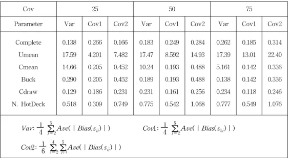
4.2. The results for the Variance-Covariance matrix under MCAR The parameters in variance-covariance matrix are grouped into 3 parts like Figure 2. `Var' is a part for the variances for the incomplete variables X₂, X₃, X₄, X₅. The covariances can be divided by two parts because X₁ is fully observed. 'Cov1' is a part for the covariances between X₁ and other incomplete variables. 'Cov2' is a part for the covariances among incomplete variables.

Table 4 shows biases of estimates for the variance-covariance matrix under MCAR. The values of `Var', 1

4 ∑⁵

j = 2Ave(∣Bias( s_jj)∣), are the average of 4

values of ` Ave(∣Bias( sjj)∣)' for s<sub>22</sub>,s<sub>33</sub>,s<sub>44</sub>,s<sub>55</sub>. ` Ave(∣Bias( sjj)∣)' is the average of 1000 values of ∣Bias( sjj)∣computed from 1000 data sets.

<Figure 2> 3 parameter groups in var-covariance matrix

∣Bias( s_jj)∣ is an absolute value of (sample variance of X_j - true variance of X_j) for 200 observations from the imputed data set. The values of `Cov1' and

`Cov2' are defined as similarly as those in `Var'.

`Cdraw' method has the smallest bias for all parameters in variance-covariance matrix. Umean is the worst for these parameters and Cmean is not good for

`Var'. The parameters in variance-covariance matrix are underestimated when we do 'Buck' method (Little and Rubin, 2002). This is not shown clearly in Table 1 because we use absolute value of bias.

Table 4: Biases for Var-Covariance Matrix under MCAR

Cov 25 50 75

Parameter Var Cov1 Cov2 Var Cov1 Cov2 Var Cov1 Cov2

Complete Umean Cmean Buck Cdraw N. HotDeck

0.138 17.59 14.66 0.290 0.129 0.518

0.266 4.201 0.205 0.205 0.186 0.309

0.166 7.482 0.452 0.452 0.231 0.749

0.183 17.47 10.24 0.189 0.231 0.775

0.249 8.592 0.193 0.193 0.161 0.542

0.284 14.93 0.488 0.488 0.256 1.068

0.262 17.39 5.161 0.138 0.234 0.777

0.185 13.01 0.142 0.142 0.118 0.549

0.314 22.40 0.336 0.336 0.246 1.076

Var : 14 ∑⁵

j = 2Ave(∣Bias( s_jj)∣) Cov1 : 1

4 ∑⁵

j = 2Ave(∣Bias( s_1j)∣)

Cov2 : 16 ∑⁴

i = 2∑⁵

j > iAve(∣Bias( s_ij)∣)

Table 5 shows relative variances of estimates for the variance-covariance matrix from the imputed data set with respect to variances for the variance-covariance matrix from the `Complete Data' under MCAR. Var(s<sub>ij</sub>)<sub>imp</sub> is the variance of 1000 sample variance of sij from the 1000 imputed data sets. Var(sij)<sub>comp</sub> is calculated similarly from the 1000 `Complete Data' sets with 200 fully observed units.

Table 2 shows that `Cmean' and `Buck' methods have less variation to estimate variance covariance matrix and their variations are close to true ones, but the values of `Umean' method are smaller than true variation.

Table 5: Relative Variances for Var-Covariance Matrix under MCAR

Cov 25 50 75

Parameter Var Cov1 Cov2 Var Cov1 Cov2 Var Cov1 Cov2

Umean Cmean Buck Cdraw N. HotDeck

0.930 0.931 1.229 1.417 1.367

0.841 1.206 1.206 1.342 1.268

0.714 1.379 1.379 1.693 1.580

0.841 1.057 1.204 1.362 1.309

0.835 1.124 1.124 1.212 1.179

0.722 1.235 1.235 1.421 1.356

0.841 1.093 1.132 1.228 1.206

0.828 1.053 1.503 1.094 1.076

0.719 1.101 1.101 1.180 1.161 Var : 1

4 ∑⁵

j = 2Var(sjj)imp/Var( sjj)comp

Cov1 : 1 4 ∑⁵

j = 2Var(s1j)imp/Var( s1j)comp

Cov2 : 1

6 ∑

4 i = 2∑

5

j > iVar(sij)imp/Var( sij)comp

In Table 6, MSE(mean square error) of the variance-covariance matrix under MCAR. Var(s_ij) + Ave( Bias( s_ij))² is (the variance of 1000 sij + the average of 1000 bias² for sij). Table 6 shows that 'Buck' method have smaller MSE to estimate variance-covariance matrix and 'Umean' method is getting worse when larger covariances exist because 'Umean' imputation does not consider the associations between variables.

Table 6: MSE for Var-Covariance Matrix under MCAR

Cov 25 50 75

Parameter Var Cov1 Cov2 Var Cov1 Cov2 Var Cov1 Cov2

Complete Umean Cmean Buck Cdraw N. HotDeck

103.11 412.92 323.82 127.14 146.73 141.66

55.22 65.05 66.63 66.63 74.24 69.79

53.54 94.19 74.03 74.03 90.59 85.13

104.17 410.71 221.63 125.66 142.33 137.33

65.99 133.39

74.20 74.20 80.05 78.11

64.51 269.5 79.90 79.90 91.66 88.62

106.09 409.81 144.28 120.10 130.47 128.64

82.77 248.3 87.12 87.12 90.54 89.31

83.25 561.8 91.72 91.72 98.19 97.74 Var : 1

4 ∑

5

j = 2Var( sjj) + ( Bias( sjj))² Cov1 : 1

4 ∑⁵

j = 2Var( s_1j) + ( Bias( s_1j))² Cov2 : 1

6 ∑

4 i = 2∑

5

j > iVar( sij) + ( Bias( sij))²

4.3 Comparison between MCAR and MAR

The simulation results for just `Cov=75' are shown because the results do not

much differ for 'Cov=25' and 'Cov=50'. All results of comparison MSE between MCAR and MAR in Table 7 and 8 show that Umean method does not work for all parameters and other methods do work like MCAR for all parameters. 'Buck' method is the most preferred one like MCAR for all parameters when we examine MSE.

Table 7: Comparison between MCAR and MAR for MSE of the Mean

Method MCAR, Cov=75 MAR, Cov=75

Complete Umean Cmean, Buck

Cdraw N. HotDeck

0.5019 0.6024 0.5333 0.5592 0.5685

0.5019 1.4648 0.5440 0.5721 0.5876 MSE : 1

4 ∑

5

j = 2Var( X_j) + Ave( Bias( X_j))² Table 8: Comparison between MCAR and MAR for MSE of the Var-covariance matrix

MCAR, Cov=75 MAR, Cov=75

Parameter Var Cov1 Cov2 Var Cov1 Cov2

Complete Umean Cmean Buck Cdraw N. HotDeck

106.09 409.00 144.28 120.10 130.47 128.64

82.77 248.06

87.12 87.12 90.54 89.31

83.25 625.15

91.72 91.72 98.19 97.74

106.09 613.12 148.93 124.86 136.75 138.79

82.77 489.94

90.27 90.27 94.04 94.31

83.25 832.48

94.77 94.77 101.75 102.96 Var : 1

4 ∑

5

j = 2Var( sjj) + ( Bias( sjj))²

Cov1 : 1 4 ∑⁵

j = 2Var( s_1j) + ( Bias( s_1j))²

Cov2 : 1 6 ∑⁴

i = 2∑⁵

j > iVar( sij) + ( Bias( sij))²

5. Conclusion

When we consider just MSE of the estimates, the 'Buck' method is the most preferred one for all cases and `Cdraw' and `N. HotDeck' are not bad in general.

If we are interested in just bias of the estimates, `Cdraw' is the most preferred one. We can conclude the simulation results for each parameter as following:

(a) Mean: All methods seem to be appropriate. `Cdraw' has less bias to estimate mean vectors. `Cmean(Buck)' is the preferred method when we consider the variation and MSE. Correlations between variables are getting larger, the performance of imputation is getting better.

(b) Variances: `Umean' and `Cmean' are not appropriate to estimate variances because these two methods underestimate variances of the variables by too large an amount. `Cdraw' is the preferred method when we are interested in the point estimates of variances. `Buck' method is the most preferred one when we consider the variation and MSE, but `Buck' method still tends to underestimate variances of the variables.

(c) Covariances: `Umean' is not appropriate to estimate covariances. `Cdraw' can be the best on the biases to estimate covariances and `Cmean(Buck)' tends to underestimate the covariances between two variables missing together. `Buck' method is the most preferred one when we consider the variation and MSE.

`Buck' method is generally preferred among single imputation methods to estimate mean and covariance matrix when we assume the missing variables have linear regression on the observed variables. If we consider just biases, `Cdraw' can be the best among single imputation methods especially when many cases are missing together on more than two variables. `Cdraw' and `N. HotDeck' are not bad in general. We can use `Umean' if the point estimation of mean are our purpose and there are strong evidence of MCAR. Otherwise, `Umean‘ method is not recommended to use. `Cmean’ is not a good choice if you are interested in the estimation of variances of the variables or correlations between the variables.

References

1. Buck, S. F. (1960). Amethod of estimation of missing values in

multivariate data suitable for use with an electronic computer, Journal of the Royal Statistical Society, Series B 22, 302-306

2. Little, R. J. A. and Rubin, D. B. (2002). Statistical analysis with missing data, J. Wiley & Sons, New York.

3. Rubin, D. B. (1976). Inference and missing data, Biometrika, 63, 581-592.

[ received date : Jul. 2004, accepted date : Oct. 2004 ]