Vol. 20, No. 2, pp. 5-16, April 2016
Free Vibration Analysis of Axisymmetric Conical Shell
Myung-Soo Choi*, Dong-Jun Yeo** and Takahiro Kondou***†
(Received 1 September 2015, Revised 29 March 2016, Accepted 29 March 2016)
Abstract: Generally, methods using transfer techniques, like the transfer matrix method and the transfer stiffness coefficient method, find natural frequencies using the sign change of frequency determinants in searching frequency region. However, these methods may omit some natural frequencies when the initial frequency interval is large. The Sylvester-transfer stiffness coefficient method (“S-TSCM”) can always obtain all natural frequencies in the searching frequency region even though the initial frequency interval is large. Because the S-TSCM obtain natural frequencies using the number of natural frequencies existing under a searching frequency. In this paper, the algorithm for the free vibration analysis of axisymmetric conical shells was formulated with S-TSCM. The effectiveness of S-TSCM was verified by comparing numerical results of S-TSCM with those of other methods when analyzing free vibration in two computational models: a truncated conical shell and a complete (not truncated) conical shell.
Key Words:Axisymmetric conical shells, Free vibration, Sylvester’s inertia theorem, Transfer stiffness coefficient method, Transfer matrix method, Finite element method
***†Takahiro Kondou(corresponding author) : Department of Mechanical Engineering, Kyushu University.
E-mail : [email protected], Tel : +81-92-802-3193
*Myung-Soo Choi : Department of Maritime Police Science, Chonnam National University.
**Dong-Jun Yeo : Faculty of Marine Technology, Chonnam National University.
1. Introduction
From loud speakers to aerospace structures, conical shells have been used in many industrial fields. For the free vibration of these conical shells, many researchers have studied a variety of methods, for examples, the Rayleigh-Ritz method1), the finite element method2), the transfer matrix method3), and the transfer influence coefficient method4).
Recently, the most engineers and researchers
have used the finite element method for the free vibration of shell structures, because this method can readily analyze a variety of shell structures using various shell elements. However, generally, the computational results of the vibration analysis for a structure by the finite element method are excellent if the structure is divided into a number of elements in the modeling. Thus, if we model the conical shell as an analytical model with a number of shell elements to obtain accurate natural frequencies and modes, the finite element method requires a large memory and a long time in the computational process.
We suggested a new method to significantly reduce computational time and memory without omitting the natural frequencies in the free vibration analysis of beam structures5). The algorithm was developed from a combination of Sylvester’s inertia theorem6) and the transfer
stiffness coefficient method7). It is referred to as the “Sylvester-transfer stiffness coefficient method”
(S-TSCM). Because S-TSCM can compute the number of natural frequencies existing under the searching frequency, S-TSCM can always find all natural frequencies in searching frequency region even though the initial frequency interval is large.
Thus, S-TSCM can carry out a free vibration analysis stably and quickly.
In this paper, an algorithm for the free vibration analysis of axisymmetric conical shells was formulated using S-TSCM. The effectiveness of S-TSCM was assessed by comparing computational results obtained by S-TSCM with those obtained by other methods when analyzing the free vibration of two computational models: a truncated conical shell and a complete (not truncated) conical shell.
2. Algorithms
2.1 Analytical model
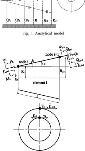
Fig. 1 shows an analytical model for an axisymmetric conical shell with elastic support springs. When the conical shell is divided into n truncated conical shell elements, the conical shell has total n+1 nodes.
When analyzing the vibration of the axisymmetric conical shell, each node has four degrees-of-freedom. The nodal displacement vector (d ) is composed of meridian, circumferential, and normal displacements ( ) and an angular displacement ( ). The nodal force vector ( f ) consists of three forces ( ) and a bending moment (). The right superscript T indicates transposition. s is the local coordinate along meridian direction.
Fig. 1 Analytical model
Fig. 2 Truncated conical shell element
If some nodes of the analytical model have elastic support springs, they are modeled with four elastic springs per node. The four springs consist of meridian, circumferential, normal springs, and a rotational spring. We denote their constants as
and .
In the transfer stiffness coefficient method7), the boundary conditions at the left and right ends of the analytical model are modeled as the elastic
support springs of the first node (node 1) and the last node (node n+1).
2.2 FE-TSCM
The finite element-transfer stiffness coefficient method (FE-TSCM)8) was developed by a combination of the modeling technique of the finite element method and the transfer technique of the transfer stiffness coefficient method to analyze the vibration of structures efficiently.
In this paper, the subscript i means the physical quantities of node i or the i-th truncated conical shell element, and the symbols with and without the symbol ‘–’ denote the physical quantities at the left side of node i (the right end of the (i-1)-th truncated conical shell element) and the right side of node i (the left end of the i-th truncated conical shell element).
The positive directions of forces and displacements of both ends of the i-th truncated conical shell element are shown in Fig. 2. The relationships between the force and the displacement vectors at the left and right sides of node i are defined as follows, making use of the dynamic stiffness coefficient matrices S and S (size: 4 × 4, symmetric) :
f Sd, (1)
f Sd, (2)
where f
and f are the force vectors of the left and right sides of node i, respectively, d is the displacement vector of node i.
If node i has elastic support spring, the balance of the forces and moments on both sides of node i yields
f f Pd ⋯ , (3)
where
P
. (4)
We can derive the matrix S from Eqs. (1)-(3) as follows :
S S P i ⋯ n . (5) Eq. (5) is called the point transmission rule to obtain the dynamic stiffness coefficient matrix S at the right side of node i from S at the left side of node i.
When the analytical model vibrates at frequency
, the relations between the force vector and the displacement vector at the left and right ends of the i–th truncated conical shell element (Fig. 2) are defined as follows by making use of the submatrices (A, B, and C) of the element dynamic stiffness matrix which is derived from the mass and stiffness matrices of the i-th truncated conical shell element9).
ff
A B
B C
dd
, (6) We can derive the matrix S from Eq. (1) in which the subscript i is changed to i+1, Eq. (2) and Eq. (6) as follows:S C BTV i ⋯ n , (7)
where
G GT S A,
V G B ⋯ . (8)
Eq. (7) is called the field transmission rule to obtain the dynamic stiffness coefficient matrix
S
at the left side of node i+1 from S at the right side of node i.
We can derive the matrix S as follows from
f and from Eqs. (2) and (3) in which the subscript i is changed to 1 :
S P. (9)
After first obtaining the matrix S from Eq.
(9), the matrix S can be finally obtained by applying Eqs. (5) and (7) successively. From
f , d ≠ , and Eq. (2) in which the subscript i is changed to n+1, the frequency equation can be driven as
S . (10)
If the bisection method10) is used to find a solution of Eq. (10), then false roots11), which are not natural frequencies, may be obtained. To overcome this problem, we compute the natural frequencies of the analytical model using the sign change of the following function,
sgn G ∙ sgn S , (11)
where is the searching frequency, which is an assumed value for the natural frequency .
After obtaining a natural frequency, the natural mode corresponding to the natural frequency can be obtained as follows. First, the displacement vector (d ) of the last node is computed from Eq. (2) in which the subscript i is changed to n+1, f S d . The displacement vector of the other nodes can be successively computed using Eq. (12) which is derived from Eqs. (2), (6), and (8). Finally, the displacement
vectors of all nodes are divided by the maximum value among all displacements to normalize the natural mode.
d Vd ⋯ . (12)
2.3 Sturm sequence method12)
The equations of motion for the undamped free vibration of a multiple degree-of-freedom system can be changed into the eigenvalue problem of matrix form,
Kd Md, (13)
where M and K are the system mass and stiffness matrices, respectively, d is the system displacement vector, and is the eigenvalue and the square of the natural circular frequency . M and K (size: 4(n+1) × 4(n+1)) for the analytical model shown in Fig. 1 can be obtained by assembling the mass and stiffness matrices (size: 4
× 4) for the n+1 truncated conical shell elements.
Generally, both M and K are real and symmetric matrices, M is the positive definite matrix, and K is the non-negative definite matrix.
d is made up of the displacement vectors of all nodes, d
d d d ⋯ d
.Eq. (13) can be changed into Sd , where S is the system dynamic stiffness matrix, S K M K M. For a nontrivial solution of Eq. (13), the characteristic equation can be driven as
S . (14)
On the other hand, S can be decomposed as LDL, where L is a lower triangular matrix in which the diagonal coefficients are all ones and D is a diagonal matrix. From Sturm’s theorem13),
the number of negative eigenvalues of S is equal to the number of negative diagonal coefficients of D.
If is the searching eigenvalue which is an assumed value for the eigenvalue , S, that is K M, can be factored into LDL, and the number of the negative coefficients in D is equal to the number of the eigenvalues that are smaller than . Thus, if is the square of , the number of the negative coefficients in D is equal to that of the natural circular frequencies that are smaller than .
2.4 S-TSCM
The system dynamic stiffness matrix S (size:
4(n+1) × 4(n+1)) for the analytical model of Fig.
1 can be expressed in detail by the matrices A, B, C, and P (size: 4 × 4), shown in Section 2.2.
S
EB ⋯ BEB ⋯
BEB⋯
BE⋯
⋮ ⋮ ⋮ ⋮ ⋱ ⋮ ⋮
⋯ E B
BE
,
E P A S A G
E C P A i ⋯ n
E C P
(15)
As shown in Eq. (16), if the symmetric matrix S is multiplied by the nonsingular matrices L and L, we can obtain the matrix Q.
Q LSL (16)
where
L LL L ⋯ L,
L
I ⋯ V I ⋯
I ⋯
I ⋯
⋮ ⋮ ⋮ ⋮ ⋱ ⋮ ⋮
⋯ I
⋯ I ,
L
I ⋯
I ⋯
V I ⋯
I ⋯
⋮ ⋮ ⋮ ⋮ ⋱ ⋮ ⋮
⋯ I
⋯ I ,
L
I ⋯
I ⋯
I ⋯
I ⋯
⋮ ⋮ ⋮ ⋮ ⋱ ⋮ ⋮
⋯ I
⋯ V I ,
Q
G ⋯
G ⋯
G ⋯
G⋯
⋮ ⋮ ⋮ ⋮ ⋱ ⋮ ⋮
⋯ Gn
⋯ Sn
, (17)
the matrices I and denote an identity matrix and a zero matrix, respectively, and the matrix V in the matrix L is equal to Eq. (8).
Because S and Q are congruent, S and Q have the same inertia, which means the numbers of positive, zero, and negative eigenvalues of a matrix, from Sylvester’s inertia theorem6). The eigenvalues of the matrix Q are equal to those that gather all eigenvalues of the matrices G, G, …, G, and S , because the matrix Q is the block diagonal matrix. Thus, the total numbers
of positive, zero, and negative eigenvalues of the matrices G, G, …, G, and S are equal to those of the system dynamic stiffness matrix S.
If is the searching eigenvalue, which is an assumed value for the eigenvalue , the total number of negative eigenvalues of the matrices G, G, …, G, and S is equal to the number of the eigenvalues that are smaller than . When the searching eigenvalue is the square of , the total number of negative eigenvalues of the matrices G, G, …, G, and S is equal to that of the natural circular frequencies that are smaller than
. While the Sylvester-transfer stiffness coefficient method computes the nodal dynamic stiffness coefficient matrices successively from node 1 to node n+1 by the transmission rules shown in Section 2.2, the natural frequencies are computed by searching the change of the value in the following function,
G S , (18)
where the function A determines the number of negative eigenvalues of the matrix A, and is the searching eigenvalue and the square of the searching frequency . From the bisection method10) and Eq. (18), the Sylvester-transfer stiffness coefficient method can always find all the natural frequencies in searching region, regardless of the initial frequency interval.
3. Numerical results
Computer programs for the free vibration analysis of the axisymmetric conical shells were created using the Sturm sequence method (SSM)12) introducing the bisection method, the finite
element-transfer matrix method (FE-TMM)14), the finite element-transfer stiffness coefficient method (FE-TSCM)8), and the Sylvester-transfer stiffness coefficient method (S-TSCM). To verify the effectiveness of S-TSCM, numerical results obtained with S-TSCM were compared with those obtained by SSM, FE-TMM, FE-TSCM and Irie’s method3), when analyzing the free vibration of two computational models, a truncated conical shell and a complete conical shell, on a personal computer (Intel Core i7-3770 [email protected], 3.48 GB RAM).
In Tables, numbers in parentheses indicate the number of truncated conical shell elements used in the modeling process. For example, (50) in Table means that a conical shell consists of 50 truncated conical shell elements. In tables, a dash means that the natural frequency could not be found. In tables, n and m are a circumferential wave number and the order of natural frequency, respectively.
3.1 Truncated conical shell
As shown in Fig. 3, the first computation model (computation model I) is a truncated conical shell with constant thickness. The length and thickness of the truncated conical shell are 1.5 m and 1.732 cm, the semi-vertex angle is 60°, and the radii of the left and right ends are 0.433 m and 1.732 m, respectively. The physical parameters of the truncated conical shell are: mass density 7850 kg/m3, Young’s modulus 200 GPa, and Poisson’s ratio 0.3.
When the truncated conical shell was divided into 5, 10, and 50 truncated conical shell elements, the natural frequencies were computed by SSM, FE-TMM, FE-TSCM, and STSCM. When the initial frequency interval, Δf, for finding natural frequencies was 1 Hz in the four methods, Table 1 shows the first natural frequencies of
Fig. 3 Computational model I
Table 1 First natural frequencies [Hz] of computational model I (Δf = 1 Hz)
n m
SSM FE-TMM FE-TSCM S-TSCM
(5)
SSM FE-TMM FE-TSCM S-TSCM
(10)
SSM FE-TMM FE-TSCM S-TSCM
(50)
Irie’s method
0 1 326.3 325.2 324.8 324.8
1 1 295.9 294.7 294.3 294.3
2 1 228.9 226.9 226.3 226.4
3 1 179.2 176.4 175.6 175.7
computational model I under four circumferential wave numbers (n = 0, 1, 2, 3). Natural frequencies obtained by S-TSCM coincided with those obtained by SSM, FE-TMM, and FE-TSCM.
Natural frequencies obtained by the four methods were similar to those obtained by Irie’s method3). In particular, when the truncated conical shell was divided into many elements, the natural frequencies of the four methods approached those of Irie’s method. The reason is that the four methods use discrete systems in modeling, whereas Irie’s method uses a continuous system.
When the initial frequency interval was 1 Hz, 10 Hz, and 100 Hz, the lowest five natural frequencies under four circumferential wave numbers (n = 0, 1, 2, 3) were computed by SSM, FE-TMM, FE-TSCM, and S-TSCM. When the truncated conical shell was divided into 50
Table 2 Lowest five natural frequencies [Hz] of computational model I
n m
SSM FE-TMM FE-TSCM S-TSCM
(50)
SSM FE-TMM FE-TSCM S-TSCM
(50)
FE-TMM FE-TSCM
(50)
SSM
S-TSCM (50) Δf=1Hz Δf=10Hz Δf=100Hz Δf=100Hz
0 1 2 3 4 5
324.8 387.8 479.1 581.9 721.4
324.8 387.8 479.1 581.9 721.4
—
— 479.1 581.9 721.4
324.8 387.8 479.1 581.9 721.4
1 1 2 3 4 5
294.3 364.3 456.2 569.5 714.9
294.3 364.3 456.2 569.5 714.9
294.3 364.3 456.2 569.5 714.9
294.3 364.3 456.2 569.5 714.9
2 1 2 3 4 5
226.3 329.1 425.4 550.1 706.6
226.3 329.1 425.4 550.1 706.6
226.3
―
― 550.1 706.6
226.3 329.1 425.4 550.1 706.6
3 1 2 3 4 5
175.6 293.5 403.5 538.7 706.2
175.6 293.5 403.5 538.7 706.2
175.6 293.5 403.5 538.7 706.2
175.6 293.5 403.5 538.7 706.2
truncated conical shell elements, Table 2 shows the lowest five natural frequencies of computational model I under four circumferential wave numbers (n = 0, 1, 2, 3) by the four programs. When the initial frequency intervals were 1 Hz and 10 Hz, the lowest five natural frequencies computed by SSM, FE-TMM, and FE-TSCM coincided with those computed by S-TSCM. When the initial frequency interval was 100 Hz, SSM and S-TSCM found the lowest five natural frequencies.
However, FE-TMM(50) and FE-TSCM(50) could not find several natural frequencies when the circumferential wave numbers were 0 and 2.
Table 3 Results of Eq. (11) and Eq. (18) for computational model I (Δf = 100 Hz) Searching
frequency [Hz]
FE-TSCM (50)
S-TSCM (50)
0 + 0
100 + 0
200 + 0
300 + 0
400 + 2
500 - 3
600 + 4
700 + 4
800 - 5
Table 4 Results of Eq. (11) and Eq. (18) for computational model I (Δf = 10 Hz) Searching
frequency [Hz]
FE-TSCM (50)
S-TSCM (50)
300 + 0
310 + 0
320 + 0
330 - 1
340 - 1
350 - 1
360 - 1
370 - 1
380 - 1
390 + 2
400 + 2
When the circumferential wave number was 0 and the initial frequency interval was 100 Hz, Table 3 shows the results of Eq. (11) and Eq.
(18). From Table 3, we know that FE-TSCM could not find the first and second natural frequencies (324.8 and 387.8 Hz), because the sign of the Eq. (11) at a frequency of 300 Hz is the same as the sign of the Eq. (11) at a frequency of 400 Hz. However, we confirmed that
S-TSCM could find the two natural frequencies from Tables 3 and 4 although the initial frequency interval was 100 Hz.
Table 5 shows the computational time according to the initial frequency intervals for finding the lowest five natural frequencies under four circumferential wave numbers. From Table 5, we know that the computational time is reduced when the initial frequency interval is increased and S-TSCM is superior to SSM in terms of computational time.
We computed the natural modes of computation model I. The results of S-TSCM agreed well with those of other methods. Fig. 4 shows the first, second, and third natural modes of computation model I calculated by S-TSCM when the circumferential wave number was 0.
When computational model I is modeled as the 50 truncated conical shell elements and the degrees-of-freedom of each node is four, the total degrees-of-freedom of the system is 204. The sizes of the system dynamic stiffness coefficient matrix of SSM and the nodal dynamic stiffness coefficient matrix of S-TSCM are 204 × 204 and 4 × 4, respectively. Therefore, we know that S-TSCM is superior to SSM in terms of the management of computation memory, because S-TSCM uses the transfer technique.
Table 5 Computational time [s] of computational model I according to initial frequency interval
Initial frequency
interval (Δf)
SSM (50)
FE-TMM (50)
FE-TSCM (50)
S-TSCM (50)
1 Hz 87.14 15.57 12.76 12.74
10 Hz 17.14 3.09 2.52 2.51
100 Hz 11.85 2.19 1.77 1.74
(a) n=0, m=1
(b) n =0, m=2
(c) n=0, m=3
Fig. 4 Natural modes of computational model I
3.2 Perfect conical shell
The computation model II is a perfect conical shell with constant thickness (Fig. 5). The length and thickness of the conical shell are 2 m and 1 cm, the semi-vertex angle is 30°, and the radius of the right end is 1 m. The physical parameters coincide with those in computational model I.
When the perfect conical shell was divided into 5, 10, and 50 axisymmetric truncated conical shell elements, the natural frequencies were computed by SSM, FE-TMM, FETSCM, and S-TSCM. When the initial frequency interval was 1 Hz, Table 6 shows the first natural frequencies under five circumferential wave numbers (n = 0, 1, 2, 3, 4).
The natural frequencies obtained by S-TSCM coincided with those obtained by SSM and FE-TSCM. There were some problems in FE-TMM. When the circumferential wave number
Fig. 5 Computational model II
Table 6 First natural frequencies [Hz] of computational model II (Δf = 1 Hz)
n m
SSM FE-TMM FE-TSCM S-TSCM
(5)
SSM FE-TSCM
S-TSCM (10)
FE-TMM
(10)
SSM FE-TSCM
S-TSCM (50)
0 1 837.1 811.1 811.3 805.7
1 1 509.5 507.2 508.8 506.7
2 1 311.6 301.9 301.2 291.6
3 1 252.5 229.2 226.7 223.9
4 1 231.8 216.5 — 211.7
Table 7 Lowest five natural frequencies [Hz] of computational model II
n m
SSM FE-TSCM
S-TSCM (50)
SSM FE-TSCM
S-TSCM (50)
FE-TSCM (50)
SSM S-TSCM
(50) Δf = 1 Hz Δf = 10 HzΔf = 100HzΔf = 100Hz
0 1 2 3 4 5
805.7 896.5 915.5 954.6 1023
805.7 896.5 915.5 954.6 1023
―
―
―
― 1023
805.7 896.5 915.5 954.6 1023
1 1 2 3 4 5
506.7 722.3 814.1 915.0 1017
506.7 722.3 814.1 915.0 1017
506.7 722.3 814.1 915.0 1017
506.7 722.3 814.1 915.0 1017
2 1 2 3 4 5
291.6 514.8 717.6 833.5 939.1
291.6 514.8 717.6 833.5 939.1
291.6 514.8 717.6 833.5 939.1
291.6 514.8 717.6 833.5 939.1
3 1 2 3 4 5
223.9 410.8 602.2 747.3 864.4
223.9 410.8 602.2 747.3 864.4
223.9 410.8 602.2 747.3 864.4
223.9 410.8 602.2 747.3 864.4
4 1 2 3 4 5
211.7 375.2 546.5 695.1 824.1
211.7 375.2 546.5 695.1 824.1
211.7 375.2 546.5 695.1 824.1
211.7 375.2 546.5 695.1 824.1
Table 8 Computational time [s] of computational model II according to initial frequency interval (Δf)
Δf SSM
(50) FE-TSCM
(50) S-TSCM (50)
1 Hz 140.18 20.52 20.57
10 Hz 24.42 3.55 3.58
100 Hz 15.01 2.20 2.20
was four, the first natural frequency could not be found by FE-TMM(10). FE-TMM(50) produced numerically unstable and meaningless results.
When the initial frequency intervals were 1 Hz, 10 Hz, and 100 Hz, the lowest five natural frequencies under five circumferential wave numbers (n = 0, 1, 2, 3, 4) were computed by SSM, FE-TSCM, and S-TSCM. When the perfect conical shell was divided into 50 truncated conical shell elements, Table 7 shows the lowest five natural frequencies of computational model II computed by the three methods. When the initial frequency intervals were 1 Hz and 10 Hz, the lowest five natural frequencies computed by SSM and FE-TSCM coincided with those computed by S-TSCM. When the initial frequency interval was 100 Hz, SSM and S-TSCM could find the lowest five natural frequencies. However, FE-TSCM could not find four natural frequencies (805.7, 896.5, 915.5, and 954.6 Hz) when the circumferential wave number was 0.
Table 8 shows the computational time according to the initial frequency intervals for finding the lowest five natural frequencies under five circumferential wave numbers. From Table 8, we can see that the computational time was reduced when the initial frequency interval was increased and S-TSCM was superior to SSM in terms of computational time. Thus, we can confirm that S-TSCM is stable and fast in finding the natural frequencies because it is possible to set a large value for the initial frequency interval when finding natural frequencies.
We computed the natural modes of computational model II. The results of S-TSCM agreed well with those of other methods. Fig. 6 shows the first, second, and third natural modes of computational model II calculated by S-TSCM when the circumferential wave number is zero.
(a) n=0, m=1
(b) n=0, m=2
(c) n=0, m=3
Fig. 6 Natural modes of computational model II
4. Conclusions
In this paper, an algorithm for the free vibration analysis of axisymmetric conical shells was formulated with the Sylvester-transfer stiffness coefficient method.
The computation results of the free vibration analysis for the truncated conical shell and the perfect conical shell by the Sylvester-transfer stiffness coefficient method were compared with those obtained by the Sturm sequence method, the finite element-transfer matrix method, the finite element-transfer stiffness coefficient method, and so forth.
We confirmed that the finite element-transfer matrix method and the finite element-transfer stiffness coefficient method may omit some natural frequencies according to the initial frequency interval, when analyzing free vibration of axisymmetric conical shells. On the other hand, the Sylvester -transfer stiffness coefficient method can find stably and conveniently all natural frequencies in the searching frequency region. In terms of computational time and memory, the Sylvester -transfer stiffness coefficient method was superior to the Sturm sequence method.
References
1. H. Saunders, E. J. Wisniewski and P. R.
Paslay, 1960, “Vibrations of Conical Shells”, Journal of the Acoustical Society of America, Vol. 32, No. 6, pp. 765-772.
2. S. K. Sen and P. L. Gould, 1974, “Free Vibration of Shells of Revolution Using FEM”, Journal of the Engineering Mechanics Division, American Society of Civil Engineers, Vol. 100, pp. 283-303.
3. T. Irie, G. Yamada and K. Tanaka, 1984,
“Natural Frequencies of Truncated Conical
Shells”, Journal of Sound and Vibration, Vol.
92, No. 3, pp. 447-453.
4. D. J. Yeo, 2005, “Development of Vibrational Analysis Algorithm for Truncated Conical Shells”, Journal of the Korean Society for Power System Engineering, Vol. 9, No. 3, pp. 58-65.
5. M. Choi, T. Kondou and Y. Bonkobara, 2012,
“Development of Free Vibration Analysis Algorithm for Beam Structures by Combining Sylvester’s Inertia Theorem and Transfer Stiffness Coefficient Method”, Journal of Science and Technology, Vol. 26, No. 1, pp. 11-19.
6. J. W. Demmel, 1997, “Applied Numerical Linear Algebra”, Siam, Philadelphia, pp. 202-203.
7. T. Kondou, T. Ayabe and A. Sueoka, 1997,
“Transfer Stiffness Coefficient Method Combined with Concept of Substructure Synthesis Method (Linear Free and Forced Vibration Analyses of a Straight-Line Beam Structure)”, JSME International Journal (Series C), Vol. 40, pp.
187-196.
8. M. S. Choi, D. J. Yeo, J. H. Byun, J. J. Suh and J. K. Yang, 2007, “In-Plane Vibration Analysis of General Plates”, Journal of the Korean Society for Power System Engineering, Vol. 11, No. 4, pp. 78-85.
9. C. T. F. Ross, 1984, “Finite Element Programs for Axisymmetric Problems in Engineering”, Ellis Horwood Limited, Chichester, pp. 105-115.
10. W. H. Press, S. A. Teukolsky, W. T. Vetterling and B. P. Flannery, 2007, “Numerical Recipes, The Art of Scientific Computing (3rd ed.)”, Cambridge University Press, New York, pp.
447-449.
11. A. Sueoka, T. Kondou, D. H. Moon and K.
Yamasita, 1998, “A Method of Vibrational Analysis Using a Personal Computer (A Suggested Transfer Influence Coefficient Method)”, The Memoirs of the Faculty of Engineering, Kyushu University, Vol. 48, No.
1, pp. 31-46.
12. JSME, 1998, “JSME Computational Mechanics Handbook, Vol. I, Finite Element Method (Structure Part)”, Maruzen, Tokyo, pp. 38.
13. A. Y. T. Leung, 1993, “Dynamic Stiffness and Substructures”, Springer-Verlag, London, pp. 42-44.
14. M. A. Dokainish, 1972, “A new approach for plate vibration: combination of transfer matrix and finite element technique”, ASME Journal of Engineering for Industry, Vol. 94, pp.
526-530.
![Table 1 First natural frequencies [Hz] of computational model I ( Δ f = 1 Hz) n m SSM FE-TMM FE-TSCM S-TSCM (5) SSM FE-TMM FE-TSCMS-TSCM(10) SSM FE-TMM FE-TSCMS-TSCM(50) Irie’s method 0 1 326.3 325.2 324.8 324.8 1 1 295.9 294.7 294.3 294.3 2 1 228.9 226.9](https://thumb-ap.123doks.com/thumbv2/123dokinfo/5260722.631433/7.808.403.709.140.664/table-natural-frequencies-computational-model-tscms-tscms-method.webp)
![Table 4 Results of Eq. (11) and Eq. (18) for computational model I (Δ f = 10 Hz) Searching frequency [Hz] FE-TSCM(50) S-TSCM(50) 300 + 0 310 + 0 320 + 0 330 - 1 340 - 1 350 - 1 360 - 1 370 - 1 380 - 1 390 + 2 400 + 2](https://thumb-ap.123doks.com/thumbv2/123dokinfo/5260722.631433/8.808.78.383.466.756/table-results-computational-model-searching-frequency-tscm-tscm.webp)

![Table 7 Lowest five natural frequencies [Hz] of computational model II n m SSM FE-TSCMS-TSCM (50) SSM FE-TSCMS-TSCM(50) FE-TSCM(50) SSM S-TSCM(50) Δ f = 1 Hz Δ f = 10 Hz Δ f = 100Hz Δ f = 100Hz 0 123 4 5 805.7896.5915.5954.61023 805.7896.5915.59](https://thumb-ap.123doks.com/thumbv2/123dokinfo/5260722.631433/10.808.81.379.153.769/table-lowest-natural-frequencies-computational-model-tscms-tscms.webp)

