Copyright © The Institute of Positioning, Navigation, and Timing http://www.ipnt.or.kr Print ISSN: 2288-8187 Online ISSN: 2289-0866
1. INTRODUCTION
A global navigation satellite system (GNSS) is a system that calculates user’s positioning by receiving satellite signals.
It is vulnerable to radio frequency interference because its power level is low as approximately -130 dBm received in the ground. Accordingly, several damages due to GNSS radio frequency interference have been reported in South Korea.
Reception failures were reported from 181 communication base stations, 15 civil aircrafts, and one warship in 2010, furthermore GPS reception failures were reported from 1,016 aircrafts and 317 ships due to jamming for 15 days in 2012 (Lim 2013). The damage was also reported in Korea as well as in overseas due to the disturbance of global positioning system (GPS) that guided missiles of the US army hit the unintended place during the Iraq War in 2003. In addition to the jamming signals at the L1 frequency band, radio frequency threat signals were detected in L2 and L5 frequency bands as well (Joo et al. 2011). A previous study
Analysis on Design Factors of the Optimal Adaptive Beamforming Algorithm for GNSS Anti-Jamming Receivers
Dong-Hoon Jang
1, Hyeong-Pil Kim
2, Jong-Hoon Won
2†1
R&D Center, DANAM Systems, Anyang 13930, Korea
2
Department of Electrical Engineering, Inha University, Incheon 22212, Korea
ABSTRACT
This paper analyzes the design factors for GNSS anti-jamming receiver system in which the adaptive beamforming algorithm is applied in GNSS receiver system. The design analysis factors used in this paper are divided into three: antenna, beamforming algorithm, and operation environment. This paper analyzes the above three factors and presents numerical simulation results on antenna and beamforming algorithm.
Keywords: GNSS anti-jamming, adaptive beamforming, minimum variance distortionless response, adaptive array
verified that a tone form radio frequency interference signal was detected from the center frequency in L1 band, and radio frequency threat signals, in which the center frequency of the signal was moved (sweeping form) over the entire effective frequency band of 24 MHz, were detected in both of L2 and L5 frequencies (Lim 2013).
To cope with such radio interferences, a number of studies have been conducted in GNSS receiver-related fields. The interference signals can be divided into two categories: unintentional and intentional signals (Dovis 2015). The intentional interference signals are then divided into jamming, spoofing, and meaconing according to the interference method used. Among these, a jamming technique is a technique of a reception disruption of GNSS signals by making the radiation of the interference signal output large in the same frequency band of GNSS signals.
Anti-jamming techniques are methods to cope with jamming techniques to mitigate the jamming effect on receivers.
For anti-jamming techniques, two methods can be used:
a method of null steering signals in the jamming signal direction and beamforming method that makes the receiver antenna’s radiation pattern to be directional to GNSS satellites (Sin 2013). In the null steering method, a power minimization (PM) algorithm using space-time processors is applied, and null is formed with regard to jamming signals of wide and narrow bands (Myrick 2001). The beamforming Received Jan 16, 2019 Revised Feb 19, 2019 Accepted Mar 04, 2019
†
Corresponding Author E-mail: [email protected]
Tel: +82-32-860-7406 Fax: +82-32-865-8623
Dong-Hoon Jang https://orcid.org/0000-0002-1249-4699
Hyeong-Pil Kim https://orcid.org/0000-0002-4090-9388
Jong-Hoon Won https://orcid.org/0000-0001-5258-574X
20 JPNT 8(1), 19-29 (2019)
is a one of beam steering techniques to form a beam into the specific direction (satellite signal reception direction where the satellite is located in GNSS system) by adjusting the amplitude and phase of the reception signals in the array antenna. Using this kind of beamforming methods, effects of jamming signals can be minimized and the gain of GNSS signals can be improved thereby obtaining a relatively high signal-to-noise ratio (SNR).
In the meantime, adaptive beamforming is one of the beamforming techniques, in which beams are formed actively by using algorithms. To actively form a beam, a weight is assigned adaptively to signals received in the array antenna elements. Through this, beam can be formed in a specific direction by adjusting the gain and phase of the signals appropriately. A variety of algorithms are present in the adaptive beamforming algorithm such as minimum power distortionless response (MPDR), maximum signal to interference plus noise ratio (MSINR) and blind beamforming (Harry 2002). A sample matrix inversion (SMI) algorithm and MPDR algorithm-applied techniques have been studied in the radar system to cope with jamming signals (Jang et al. 2013). For GNSS receivers with array antennas, studies on algorithm applications of minimum variance distortionless response (MVDR) and comparative analysis with Conventional beamforming algorithm have been conducted (Song 2013). A study on blind beamforming algorithm of GNSS receivers was also conducted (Zheng 2008). Generally, the performance of the MSINR algorithm is superior but its implementation is difficult whereas the MPDR algorithm is easy to implement (Harry 2002).
However, the MPDR technique requires attitude information including information on incident direction such as azimuth and elevation in regard to GNSS satellite signals, receiver’s position, and velocity. As a result, it is closely influenced by the operation environment. A study on algorithms about error factors such as instability of array antenna and environmental factors in the adaptive beamforming technique was also conducted (Vorobyov et al. 2003).
This paper analyzed the following three design factors:
antenna, beamforming weight algorithm, and user operation environment in order to design the optimal adaptive beamforming system. The antenna performance is dependent on antenna element characteristics, the number of elements, and array method. To analyze this, the design and analysis are conducted by considering the array antenna element characteristics of GNSS receivers using the high frequency structure simulator (HFSS). In addition, design and analysis on the antenna directivity according to the number of antenna elements is conducted through the HFSS. The beam width according to the number of elements is compared and
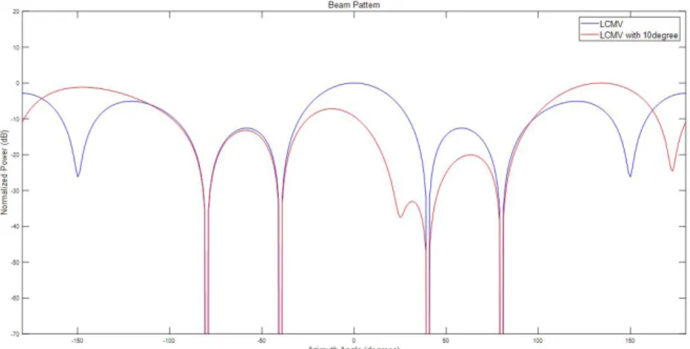
analyzed using MATLAB, just as the beamforming weight algorithm Simulations are performed for the following 4 cases such as the algorithm with the same weight, the conventional beamforming weight algorithm, the linearly constrained minimum variance (LCMV) and the MVDR beamforming weight algorithm, and the consequent results are compared and analyzed. Finally, the performance differences of attitude information providing sensors are compared and analyzed numerically according to the user operation environment. To provide attitude information, a method using a sensor and a method of fixed attitude information input can be used.
These methods that provide attitude information are applied differently according to the user operation environment, which are applied through comparison and analysis via data sheet of the sensors. Through the design factor analysis, users can consider the optimal design factors that suit the operation environment.
In the first section of this paper, a general GNSS anti- jamming receiver system is mentioned and explained using the system configuration diagram. Next, the above three design factors: antenna, weight algorithm, and operation environments are described through structures and equations. Finally, simulation results of the design factors are analyzed.
2. GNSS ANTI-JAMMING RECEIVER SYSTEM
2.1 GNSS Anti-jamming Receiver System
GNSS signals are modulated signals of carrier, code, and navigation message. The navigation message contains ephemeris data, used to calculate the position of each satellite in orbit, information related to the time and all GNSS satellites orbital information, called almanac (Kaplan &
Hegarty 2006).
The configuration of GNSS receiver system is shown in
Fig. 1. GNSS signals from medium Earth orbit satellites are
received by antennas. The received signals are transferred
Fig. 1. Functional block diagram of GNSS receiver system.
http://www.ipnt.or.kr to the receiver through the RF front end. The transferred
signals are converted to digital signals at a low frequency in order to be processed by software after a series of processes: amplification, down conversion to baseband or intermediate frequency, filtering to remove noises and frequencies in outside of the intended band, and analog to digital conversion by hardware. The converted digital signals are decoded through signal processing such as acquisition and tracking, and the receiver obtains fine estimated signal parameters for calculating the position solution.
Different anti-jamming techniques are applied to antenna and receiver algorithm in GNSS receiver system to cope with relevantly different jamming signals. As the performance of anti-jamming techniques becomes better, a size of the receiver system, complexity, and cost increase. For example, the more the number of array antenna elements is, the better it can cope with jamming signals generally. However, it increases the size of array antenna and computational load, which are drawbacks (Harry 2002).
The simplest method to cope with jamming signals is to use a filter. A frequency band where the jamming signals are located is blocked using a bandpass filter whose cut-off characteristic is excellent. However, this method is difficult to cope with jamming signals that have the same band with that of GNSS signals. In addition, the cut-off characteristic should be excellent if the receive band is closer even if jamming signals that have a different band from GNSS signal band are received.
The controlled reception pattern array (CRPA) technique is an anti-jamming technique to control synthesized or combined reception patterns of array antenna elements. The CRPA technique detects the direction of the jamming signal when jamming signals are introduced in an environment where satellite signals are received, and controls the gain and phase of each element in the array antenna thereby forming a null in the jamming signal direction. As the jammer size increases, the null depth decreases (Kaplan & Hegarty 2006).
There are other similar methods such as spatial time adaptive processing (STAP) algorithm or spatial frequency adaptive processing (SFAP) algorithm for anti-jamming techniques, where both techniques are for beam steering and null forming in not only spatial domain but also time or frequency domain simultaneously (Harry 2002).
2.2 Antenna
GNSS receiver antennas have a characteristic of right hand circularly polarization (RHCP) to receive GNSS signals, and its resonance frequency is designed in accordance with GNSS frequency band. On the other hand, a reflected GNSS signal
wave has a characteristic of left hand circularly polarization (LHCP). Thus, if signals that have LHCP characteristic are fairly removed, the interference due to multi-path can be minimized (Boccia et al. 2004). In addition, GNSS receiver systems are utilized in various fields such as GNSS signal control and monitoring and GNSS receivers. Although various antennas are necessary according to the use purpose, microstrip patch antennas are generally used in receivers considering the GNSS signal characteristics.
An array antenna is a set of multiple antennas connected together as a single antenna. In the array antenna, each of the single antenna is called an element of the array antenna.
The receive pattern of the radio wave radiated from each of the antenna element can be combined sophisticatedly by controlling the amplitude and phase of the receiving signals.
The effect of the interference signals can be reduced by this control (Widrow et al. 1967). In addition, sidelobes can be controlled, and the pattern of the mainlobe can be modified.
As a result, the radiation pattern is more complex than that of single antenna. The radiation pattern of the array antenna is determined by the array antenna element. The current and phase excited in each element, a distance between elements, an array method, and the number of elements are major parameters to determine the characteristics of the array antenna. Among these, the array method is generally divided into three types: linear, circular, and planar arrays according to the geometrical structure (Balanis 2005).
A linear array is an array method to use elements arrayed in the straight line. In this array, a distance between elements becomes the primary parameter. If a distance between elements is the same and the elements are placed in the same space, it is called uniform linear array (ULA). The array factor is defined as the complex-valued radiation pattern determined by the characteristics of each element and the distance of the elements. The array factor is obtained through Eq. (1) in which the array coefficient is multiplied by the electric field of single element (Harry 2002).
parameters to determine the characteristics of the array antenna. Among these, the array method is generally divided into three types: linear, circular, and planar arrays according to the geometrical structure (Balanis 2005).
A linear array is an array method to use elements arrayed in the straight line. In this array, a distance between elements becomes the primary parameter. If a distance between elements is the same and the elements are placed in the same space, it is called uniform linear array (ULA). The array factor is defined as the complex-valued radiation pattern determined by the characteristics of each element and the distance of the elements. The array factor is obtained through Eq. (1) in which the array coefficient is multiplied by the electric field of single element (Harry 2002).
∑
(1)
where AF is the array factor, refers to the weight per element toward the incident signals, and
represents the electric field of single element.
As the spacing between elements is shorter in the array antenna, elements cause mutual interference.
The interaction occurred due to this interference is called mutual coupling. Since this mutual coupling influences the array factor,the design should be taken with more attention. The mutual coupling may occur in the space because the spacing between elements is closer as mentioned above, or it may occur due to adjacent obstacles or feed line.
The antenna’s gain means a relative gain between directional and omni-directional patterns. That is, the higher the gain is, the larger the main beam’s size (dB) is in a specific direction. The directivity is a parameter that displays a shape of radiation pattern, in which the main beam is gathered in a given direction. The directivity (D) is defined as presented in Eq. (2) (Pozar 2012).
(2)
where
is the maximum value of radiation density F, and
is the total power radiated from the antenna. D is one for an omni-directional antenna, and is larger than one for a directional antenna.
2.3 Beamforming Algorithm
The beamforming or beam steering technique is a signal processing method to make a directional antenna radiation pattern. The radiation pattern of the array antenna causes constructive or destructive interference by changing an array in the array antenna or controlling a radiation pattern in a single antenna. This characteristic has been utilized in various fields such as radio, radar, and astronomy. This has also been used in anti-jamming algorithm to cope with jamming signals in GPS receiver system.
The switched beamforming technique is also called as fixed beamforming or conventional beamforming technique. The switched beam beamformer is one of the simple ways to make a beamforming algorithm that can be implemented by using a number of fixed, independent, and directional antennas or butler matrix and analog beamformer (Allen & Ghavami 2005). However, it has a drawback that beams are formed only in a pre-determined direction. Thus, users should select the most efficient direction from determined beam directions, beforehand. The switched beam beamformer is implemented by applying an algorithm such as Rotman lens, Blass matrix, and Butler matrix. Rotman lens was named after an American scientist named Walter Rotman, which implemented a function by which radar systems can see targets in multiple directions without moving an antenna system physically (Rotman 2008).
In the meantime, signals arriving from multiple directions can be received and attenuated at the same time using an adaptive beamformer. The adaptive beamforming in the anti-jamming GNSS receiver system is one of the ways that improves the signal reception performance even in poor GNSS signal reception environment (Li et al. 2008). The adaptive array collects spatial sample information in the propagated electric field domain and processes the information in the beamformer. Generally, a
(1)
where AF is the array factor, ω
*nrefers to the weight per element toward the incident signals, and e
-jkzzn) represents the electric field of single element.
As the spacing between elements is shorter in the
array antenna, elements cause mutual interference. The
interaction occurred due to this interference is called mutual
coupling. Since this mutual coupling influences the array
factor,the design should be taken with more attention. The
mutual coupling may occur in the space because the spacing
between elements is closer as mentioned above, or it may
22 JPNT 8(1), 19-29 (2019)
occur due to adjacent obstacles or feed line.
The antenna’s gain means a relative gain between directional and omni-directional patterns. That is, the higher the gain is, the larger the main beam’s size (dB) is in a specific direction. The directivity is a parameter that displays a shape of radiation pattern, in which the main beam is gathered in a given direction. The directivity (D) is defined as presented in Eq. (2) (Pozar 2012).
parameters to determine the characteristics of the array antenna. Among these, the array method is generally divided into three types: linear, circular, and planar arrays according to the geometrical structure (Balanis 2005).
A linear array is an array method to use elements arrayed in the straight line. In this array, a distance between elements becomes the primary parameter. If a distance between elements is the same and the elements are placed in the same space, it is called uniform linear array (ULA). The array factor is defined as the complex-valued radiation pattern determined by the characteristics of each element and the distance of the elements. The array factor is obtained through Eq. (1) in which the array coefficient is multiplied by the electric field of single element (Harry 2002).
∑
(1)
where AF is the array factor, refers to the weight per element toward the incident signals, and
represents the electric field of single element.
As the spacing between elements is shorter in the array antenna, elements cause mutual interference.
The interaction occurred due to this interference is called mutual coupling. Since this mutual coupling influences the array factor,the design should be taken with more attention. The mutual coupling may occur in the space because the spacing between elements is closer as mentioned above, or it may occur due to adjacent obstacles or feed line.
The antenna’s gain means a relative gain between directional and omni-directional patterns. That is, the higher the gain is, the larger the main beam’s size (dB) is in a specific direction. The directivity is a parameter that displays a shape of radiation pattern, in which the main beam is gathered in a given direction. The directivity (D) is defined as presented in Eq. (2) (Pozar 2012).
(2)
where
is the maximum value of radiation density F, and
is the total power radiated from the antenna. D is one for an omni-directional antenna, and is larger than one for a directional antenna.
2.3 Beamforming Algorithm
The beamforming or beam steering technique is a signal processing method to make a directional antenna radiation pattern. The radiation pattern of the array antenna causes constructive or destructive interference by changing an array in the array antenna or controlling a radiation pattern in a single antenna. This characteristic has been utilized in various fields such as radio, radar, and astronomy. This has also been used in anti-jamming algorithm to cope with jamming signals in GPS receiver system.
The switched beamforming technique is also called as fixed beamforming or conventional beamforming technique. The switched beam beamformer is one of the simple ways to make a beamforming algorithm that can be implemented by using a number of fixed, independent, and directional antennas or butler matrix and analog beamformer (Allen & Ghavami 2005). However, it has a drawback that beams are formed only in a pre-determined direction. Thus, users should select the most efficient direction from determined beam directions, beforehand. The switched beam beamformer is implemented by applying an algorithm such as Rotman lens, Blass matrix, and Butler matrix. Rotman lens was named after an American scientist named Walter Rotman, which implemented a function by which radar systems can see targets in multiple directions without moving an antenna system physically (Rotman 2008).
In the meantime, signals arriving from multiple directions can be received and attenuated at the same time using an adaptive beamformer. The adaptive beamforming in the anti-jamming GNSS receiver system is one of the ways that improves the signal reception performance even in poor GNSS signal reception environment (Li et al. 2008). The adaptive array collects spatial sample information in the propagated electric field domain and processes the information in the beamformer. Generally, a
(2)
where F
maxis the maximum value of radiation density F, and P
radis the total power radiated from the antenna. D is one for an omni-directional antenna, and is larger than one for a directional antenna.
2.3 Beamforming Algorithm
The beamforming or beam steering technique is a signal processing method to make a directional antenna radiation pattern. The radiation pattern of the array antenna causes constructive or destructive interference by changing an array in the array antenna or controlling a radiation pattern in a single antenna. This characteristic has been utilized in various fields such as radio, radar, and astronomy. This has also been used in anti-jamming algorithm to cope with jamming signals in GPS receiver system.
The switched beamforming technique is also called as fixed beamforming or conventional beamforming technique.
The switched beam beamformer is one of the simple ways to make a beamforming algorithm that can be implemented by using a number of fixed, independent, and directional antennas or butler matrix and analog beamformer (Allen
& Ghavami 2005). However, it has a drawback that beams are formed only in a pre-determined direction. Thus, users should select the most efficient direction from determined beam directions, beforehand. The switched beam beamformer is implemented by applying an algorithm such as Rotman lens, Blass matrix, and Butler matrix. Rotman lens was named after an American scientist named Walter Rotman, which implemented a function by which radar systems can see targets in multiple directions without moving an antenna system physically (Rotman 2008).
In the meantime, signals arriving from multiple directions can be received and attenuated at the same time using an adaptive beamformer. The adaptive beamforming in the anti-jamming GNSS receiver system is one of the ways that improves the signal reception performance even in poor GNSS signal reception environment (Li et al. 2008). The adaptive array collects spatial sample information in the propagated
electric field domain and processes the information in the beamformer. Generally, a beamformer combines the spatially sampling information from each of the elements linearly and obtains a scalar outcome time information. This method is similar with the FIR filter, in which sampling data are combined linearly. The structure of the beamformer is shown in Fig. 2. First, signals are received from each of the elements in the array antenna. The received signal forms a beam by applying a weight via adaptive algorithm. Some of the typical adaptive algorithms are Null-Steering, MVDR, minimum mean square error (MMSE), and MSINR.
The null-steering technique is the simplest adaptive beamforming technique, which can form a null with regard to various jamming signals. It is important for the null- steering technique to detect a direction of jamming signal reception. N-1 nulls can be formed where N is the number of elements in the array antenna. When a mainlobe and a region where a null is formed are very close, the performance may be degraded. In situations, where an antenna steered null is created in an undesired direction, the beam pattern gets distorted due to noise effect.
The MMSE technique requires a separate reference signal.
It is a technique to acquire an optimal weight that minimizes the difference between output and reference signals. Typical MMSE techniques are least mean square (LMS) and recursive least square (RLS).
2.4 Operating Condition
The quality of GNSS signals in anti-jamming GNSS
receiver system has a significant impact on the anti-jamming
performance. The error of anti-jamming GNSS receiver system
should be minimized to improve the quality of signals. In
the previous sections, performances were described under
Fig. 2. Structure of adaptive beamformer.
http://www.ipnt.or.kr ideal conditions without errors. However, the following
errors should be taken into consideration in real systems.
In the adaptive beamforming system, a correlation with interference signals, element characteristic errors, element array error, and weight calculation errors cause performance degradation (Godara 1997). In addition, the performance may be degraded due to small sample size or when source or array of array antenna change according to environmental factors. In particular, the adaptive system reacts sensitively to a small mismatch between estimated signal and actual beam steering vector when trained reference signals during algorithm execution are used. Thus, beamforming with wrong information of reference signals may cause the additional performance degradation. This mismatch could occur due to environmental inhomogeneities, distorted outer shape, unstable manifold correction, near-far mismatch, or problems in signal propagation (Vorobyov et al. 2003). Performance is also degraded if the information about preferred direction is inaccurate even if beams are steered accurately to the preferred angle in the adaptive beamformer where a beam width is very narrow. This type of errors is called pointing error, which can be minimized by enlarging the mainlobe width. A study reported that it was not necessary to enlarge a mainlobe width to reduce the effect of pointing error (Ponnekanti &
Sali 1996). The effect of pointing error can be minimized by applying the maximum likelihood (ML) method.
The adaptive beamforming technique has been utilized in various fields such as wireless communication, radar, sonar, microphone array speech processing, medical imaging, vehicles, and guided missiles. Since it has been utilized in various fields, it requires robustness. The research on beamforming techniques considering the robustness is underway. For robust adaptive beamforming (RAB) technique, a standard MVDR technique is applied along with the estimate of the preferred signal steering vector discovered based on some inaccurate previous information (Khabbazibasmenj et al. 2012).
Various application fields are classified into four cases according to changes in two characteristics: position and attitude. First case is the fixed position and attitude, wherethe system is not moving, and antenna movement is fixed such as positioning and geodetic surveying. Second case is the fixed position and dynamic changes in attitude. A system such as radar is located at a fixed position and the attitude of antenna changes geometrically to perform scanning. Third case is that an antenna is fixed without changes in attitude when a position moves. The final case is where there is a change in attitude while moving a position. The system moves at some velocity in an operational environment such as vehicles, ships, and missiles. The change in attitude of antenna can
be considered according to the moving path or it may be excluded in the consideration.
The above four cases require different aiding. First, when attitude and position changes are fixed, it is reasonable to directly use the previously known fixed values for the attitude and position. Second, when dynamic changes in attitude occurs at a fixed position, it is reasonable to utilize an encoder to measure changes in attitude. For example, a positioner may provide an accurate angular value without bias with regard to the rotation axis. Finally, it is generally feasible to use inertial measurement unit (IMU) in regard to position and attitude under dynamic environments. The sensor unit provides attitude information such as roll, pitch, and yaw considering the changes in velocity of moving objects. However, a bias is present in a sensor, which is a disadvantage.
3. SIMULATION
3.1 Antenna
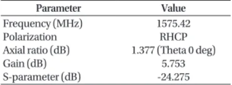
This section analyzes the directivity and array factor according to the number of antenna elements to verify the beamforming performance according to the array antenna in anti-jamming GNSS receiver system. Table 1 presents the design parameters of single patch antenna for a GNSS receiver assumed to be used in the simulation of this study.
Fig. 3 shows the three-dimensional (3D) radiation pattern when a single element antenna is designed based on the assumed design parameters in Table 1. The figure verifies that there is no significant pattern distortion since it is a single element and the gain is approximately 5.78 dB. The measured reflection loss was approximately –24 dB or smaller at 1.57542 MHz, and the measured axial ratio was approximately 1.37 dB at theta 0°.
In the same manner, when the number of elements was increased to seven in the array, a pattern of simulation result was obtained as shown in Fig. 4. Since there was no factors that incurred an interference in a single element, a pattern that was closer to a sphere was made. However, in the case of seven elements, six nulls were formed due to the interference between elements. In addition, a beam width of the mainlobe with directivity became sharp. Accordingly, the maximum
Table 1. Characteristics of designed GNSS antenna.
Parameter Value
Frequency (MHz) Polarization Axial ratio (dB) Gain (dB) S-parameter (dB)
1575.42 RHCP 1.377 (Theta 0 deg)
5.753 -24.275
24 JPNT 8(1), 19-29 (2019)
gain in the direction with directivity was approximately 12.9 dB, which was raised by 7 dB.
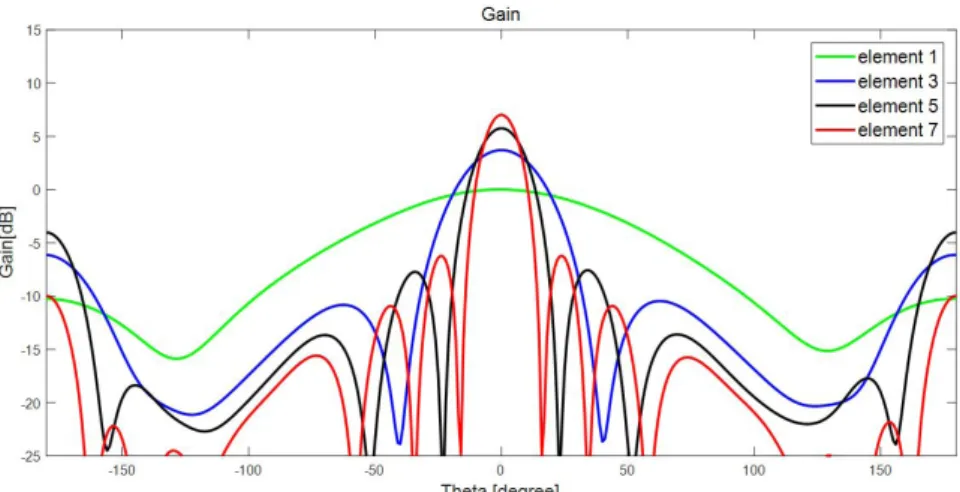
Fig. 5 shows the graph of directivity that displays the results in two-dimensional (2D) plane according to the increase in the number of elements as mentioned above. As shown in Fig. 5, with the increase in the number of antenna elements, directivity and gain are raised. If the gain was set to “0 dB”
when the number of antenna elements was one, then when the numbers of elements were three, five, and seven, the gains were raised by 4.2 dB, 6.3 dB, and 7.6 dB, respectively.
In addition, the number of nulls formed with regard to N, the number of antenna elements, was N-1, indicating that the number of nulls also increased. Furthermore, as the number of elements increased, a beam width of the main beam was formed sharply. This result showed that as the number of antenna elements increased, the number of copable interference signals also increased.
However, as the number of antenna elements increased, the following drawbacks were also present. As the number of antenna elements increased, a physical size of the antenna elements may differ according to the dielectric permittivity.
In general, a physical size increases by N times of the number of elements. Furthermore, a half wavelength is required for the spacing between antenna elements normally. Thus, if the number of antenna elements increases by N elements as shown in Fig. 6, a physical space increases by N times as well.
It means that the computation to process signals increases by N times as well, which is a shortcoming.
In general, GNSS adaptive beamforming antenna is arranged in a circular planar array shape as shown in Fig. 7 to determine the receive signal direction. In that arrangement, the disadvantage is the same that a physical size requires N Fig. 3. 3D pattern of single patch antenna.
Fig. 5. Directivity analysis according to the number of array antenna elements.
Fig. 4. 3D pattern of 7 elements array antenna.
Fig. 6. Uniform line array.
http://www.ipnt.or.kr times or larger as the number of antenna elements increases,
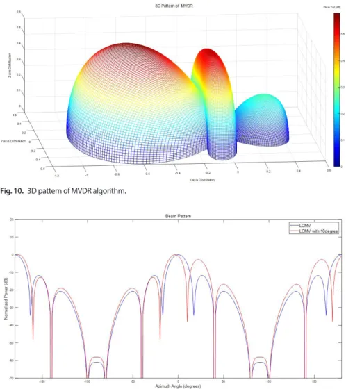
and the computation of signal processing also increases by N times. However, the 3D pattern of the array antenna varies according to the array method as shown in Fig. 8.
The antenna gain was 12.89 dB when using a linear array, and 12.43 dB using a circular planar array, showing similar results. However, the 3D pattern was more concentrated in the zenith direction in the circular planar array than in the linear array according to the antenna element arrangement.
3.2 Beamforming Algorithm
This section analyzes the beamforming weight algorithm.
Table 2 presents the conditions that are set to simulate the algorithms.
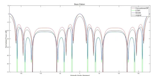
The seven single antenna elements were arranged linearly as designed in the previous section. The spacing between elements was set to 0.5 to model the half wavelength. To
compare the characteristics of the beamforming algorithms, the aforementioned beam is depicted in Fig. 9. The mainlobe was formed approximately 3 dB higher in three beamforming algorithms than that of the original beam.
This result indicated that the directivity and gain increased approximately by 3 dB. In addition, when using the LCMV and MVDR techniques, the sidelobe was controlled to have -21.61 dB, which was about 4 dB lower than that of the conventional BF algorithm whose sidelobe was simulated to -16.9 dB at -87º.
The following simulations were conducted in regard to the MVDR algorithm among the above weight algorithms. The simulation conditions were as follows: when satellite signals were received at azimuth 180° and elevation 70°, jamming
Fig. 9. Pattern comparison of beamforming algorithms.
Fig. 8. 3D pattern of 7 elements circular planar array antenna.
Fig. 7. Circular planar array.
Table 2. Simulation parameters for analysis of beamforming algorithm.
Parameter Value
C/A code (MHz) Chip rate (MHz) Sampling rate
Resolution frequency (MHz) IF frequency (MHz) Jamming signal (deg)
1.023 1/1.023 Chip rate /20
1575.42 5.115 -40, -20, 20, 40