Print ISSN: 2288-4637 / Online ISSN 2288-4645 doi:10.13106/jafeb.2019.vol6.no4.115
Does Asymmetric Relation Exist between Exchange Rate and Foreign Direct Investment in Bangladesh? Evidence from Nonlinear ARDL Analysis
Md. QAMRUZZAMAN1, Salma KARIM2, Jianguo WEI3
Received: June 18, 2019 Revised: September 16, 2019 Accepted: September 30, 2019
Abstract
The study aims to investigate the pattern of relationships such as symmetric or asymmetric, between exchange rate and foreign direct investment in Bangladesh by applying Autoregressive Distributed Lagged (ARDL) and nonlinear ARDL. In this study, we employed quarterly data for the period of 1974Q1 to 2016Q4. Data were collected and aggregated from various sources namely, Bangladesh Economic Review published by Ministry of Finance and statistical yearbook published by Bangladesh Bureau of Statistics and an annual report published by Bangladesh Bank. The relationship between exchange rate and FDI inflows attract immense interest in the recent periods, especially for developing countries’ perspective. The results of the study ascertain the long run relationship between FDI, exchange rate, monetary policy, and fiscal policy. Considering the asymmetric assumption, the findings from NARDL confirm the existence of a long-run asymmetric relationship in the empirical equation. In the long run, it is observed that positive change that is the appreciation of exchange rate against USD decrease FDI inflows and negative shocks results in grater inflows of FDI, however, the positive shocks produce higher intensity that negative shocks in Exchange rate. For directional causality, the coefficients of error correction term confirm long-run causality, in particular, bidirectional causality unveiled between FDI and exchange rate.
Keywords :Exchange Rate, FDI, ARDL, NARDL, Bangladesh
JEL Classification Code : F31, F34
1.Introduction12
The link between the exchange rate and FDI inflows in the host country is evident in the empirical literature.
Existing finance literature including Froot and Stein (1991) emphasized that the depreciation of host country currency can cause a dramatic increase of FDI inwards in the economy. Furthermore, Harris and Ravenscraft (1991)
1 First Author and Corresponding Author, Assistant Professor, School of Business and Economics, United International University, Bangladesh. [Postal Address: United City, Madani Avenue, Badda, Dhaka - 1212, Bangladesh]
Email: [email protected]
2 Professor, School of Business and Economics, United International University, Bangladesh. Email: [email protected] 3 Professor, School of Economics, Wuhan University of Technology,
China. Email: [email protected]
ⓒ Copyright: Korean Distribution Science Association (KODISA)
This is an Open Access article distributed under the terms of the Creative Commons Attribution Non-Commercial License (http://Creativecommons.org/licenses/by-nc/4.0/) which permits unrestricted noncommercial use, distribution, and reproduction in any medium, provided the original work is properly cited.
explained in their study that a depreciation of US dollar largely associated with heavy inflows of FDI in the US economy, likewise the effect of host currency depreciation attract foreign long-term investment in the form of FDI also noticed by other researchers (Dewenter, 1995; Klein &
Rosengren, 1994; Bayoumi, Bartolini, & Klein, 1996).
Empirical literature suggested that the nexus between FDI - exchange rates largely investigated with two assumptions either depreciation of host currency relatively encourage large inflows of FDI, or exchange rate fluctuation negatively influence on FDI inflows in the economy. With this study, we further moved towards investigating the existence of a nonlinear relationship between exchange rate and FDI inflows in Bangladesh by applying nonlinear Autoregressive Distributed lagged model proposed by Shin, Yu, and Greenwood-Nimmo (2014). So as to investigating FDI and exchange rate relationship in this study we decomposed both FDI and exchange rate in positive and negative shock for the purpose of unveiling the effect pattern from FDI inflows on the exchange rate and exchange rate on FDI inflows,
respectively.
As determinants of FDI inflows, several empirical studies including Liu (2010), Shapiro and Globerman (2003), and Ang (2008), exposed that host country exchange rate play a critical deterministic role in the process of inflows of FDI. Exchange rate volatility influences every core ingredients in the economy such as international trade performance, aggregated production, inflation and foreign investment in the host country. The nexus between foreign direct investment (FDI) and exchange rates, over the past couple of decades, attract immense interest among economics, researchers, and policymakers due to the direct and indirect effect of FDI inflows in the host economy is obvious, therefore ensuring stable flows FDI counties tried to maintain a favorable macroeconomic environment, most prominently stable exchange rate. Several scholars including Froot and Stein (1991), Harris and Ravenscraft (1991), and Osinubi (2010) found a positive association between inflow of FDI and exchange rate movement.
FDI flows in the economy produce spillover effect through employment generation, knowledge sharing, technological transfer, and capital accumulation. In a study, Crespo and Fontoura (2007) explained FDI influence on the economy is evident through labor mobility, backward and
forward linkages in the production along with competitiveness. Moreover, the impact of FDI on economic growth is well established and documented in the empirical studies see for an instance, (Gui-Diby, 2014; Iamsiraroj, 2016; Iamsiraroj & Ulubaşoğlu, 2015).
The effects of foreign direct investment, especially in developing countries, is multifold. As a developing nation Bangladesh persistently looking for FDI inflows over the past decade as it emerged as the key source of long-term capital and assist in domestic capital accumulation as well.
The nexus between FDI-led economic growth of Bangladesh attract researchers of exploring their fundamental relationship. In the empirical literature, we observed that the positive effects of FDI on the economic growth of Bangladesh confirmed by different researchers see for an instance, (Bari, 2013; Hussain & Haque, 2016; Adhikary, 2011; Ahamed & Tanin, 2010). The growth of FDI inflows in Bangladesh is maintaining at a stable rate of 5.11% in the year of 2018 from the prior year 2017. In the year of 2017-2018 Bangladesh received FDI of $506 million from China, $373 million from the UK, $191 million from Hong Kong, $171 million from the US, $158 million from Singapore, $135 from Norway, and $125 million from South Korea.
Table 1: FDI inflows and investment in Bangladesh
FY 2008-09 2009-10 2010-11 2012-12 2012-13 2013-14 2014-15 2015-16 2016-17
Total FDI inflows (USD Million) 961 913 779 1195 1730.63 1480.34 1833.87 2003.53 2454.81
Investment as % of GDP 26.19 6.23 27.39 28.26 28.39 28.58 28.89 29.65 30.27
Source: Economic Review of Bangladesh: Ministry of Finance (2016)
The novelty of this study relies on three distinct aspects.
First, even though a group of researchers performed empirical studies concentrating on FDI, but their focus is either on FDI impact on economic growth or determinant of FDI inflows in Bangladesh. So far our understanding, there is no such research work carried out investigating the relationship between exchange rate movement and FDI inflows in Bangladesh. With this study, we tried to fill that research gap. Second, in this study, we tried to explore relationship under both symmetric and asymmetric assumptions. The symmetric assumption was tested by applying ARDL bound testing proposed by Pesaran, Shin, and Smith (2001) and the asymmetric relationship was investigated by applying newly proposed Nonlinear ARDL by Shin et al. (2014). ARDL bounds testing approach confirmed the existence of long-run cointegration between FDI and exchange rate. Furthermore, non-linear ARDL confirmed asymmetric effects exist between FDI inflows and exchange rate both in the short – run and long – run, which is applicable in both non-linear ARDL model where both FDI and exchange rate were considered as the dependent variable in the equation.
The remaining section of this paper includes. Section 2 deals with empirical literature reviews. Section 3 contains data and methodology for empirical estimation. Section 4 describes the analysis and interpretation. Section 5 reports
the study findings and conclusion.
2. Theoretical Understanding and Literature Review
In the 1970s and 1980s, the linkages between FDI and exchange rates emerged as one of the key issues which are investigated in empirical studies see, (Kohlhagen, 1977;
Cushman, 1985). With the connection of explaining the relationship between FDI and exchange rates, numbers of theories emerged, however, predominately two theories were considered; proposed by Blonigen (1997) and Froot and Stein (1991). The imperfect capital market, according to Froot and Stein (1991) assumes that the cost of capital accumulation from external sources is higher than raising capital from internal sources. As a result, depreciation of host country currency would create positive motivation for foreign investors with positive effects on their wealth. The imperfect capital market approach, therefore, argued that the exchange rate operates on the wealth effects of FDI. For the reason, a depreciation of the host currency exchange rate increase inflows of FDI.
Over the past decades, the world experienced economic integration through the liberalization of international trade
by allowing free movement of goods and service (Ahmad &
Harnhirun, 1996) and flows of capital in the form of Foreign Direct Investment (Lipsey et al., 1999) across the country. In particular, FDI is more stable sources of capital flows in developing nations that portfolio investment (Lipsey, Feenstra, Hahn, & Hatsopoulos, 1999), it assists in expanding production possibilities and through technological slipover (Borensztein & De Gregorio, 1995).
However, researchers put immense interest on explaining FDI-led economic growth hypothesis and a large number of empirical studies, either considering panel data or country- specific time-series information, confirmed the existence of long-run relationship, see for an instance (Alvarado, Iñiguez,
& Ponce, 2017; Ericsson, 2001; Umoh, Jacob, & Chuku, 2012). With the same intention, Howitt and Aghion (1998) explained that economic growth directly linked to innovation that is the key outcome from technological advancement in the economy. They also argued that the technology integration process in the economy could accelerate through inflows of FDI and international trade collaboration.
The strong inflows of FDI in the developing economy play a crucial role in achieving sustainable economic growth.
It is because FDI increase venture capital for domestic investment, enhance the level of productivity, and technological progress along with managerial expertise in the operation (Pradhan, 2009). In a study, Borensztein, De Gregorio, and Lee (1998) suggested that FDI established a bridge between technology transfer and economic growth.
Technological transfer increase efficiency in production through wastage reduction and productivity improvement (Anwar & Nguyen, 2010). Therefore, FDI treated as an essential vehicle for domestic growth in developing countries (Qamruzzaman, 2015).
FDI inflows are influenced by macroeconomic indicators, especially exchange rate volatility influences at most (Goldberg, 2009). Exchange rate fluctuation affects FDI in two ways. First, the devaluation of host currency reduces the cost of production relative to foreign investors. Second, produce localization of advantages (Phillips & Ahmadi‐
Esfahani, 2008). Empirical studies also advocate FDI inflows can affect money supply in the economy. Finance scholars including Clarke and Ioannidis (1994) and Resende (2008) suggested aggregate money supply in the economy attract foreign investors. In a study, Pain and Van Welsum (2003) argued that the exchange rate impact on the flows of FDI varies across the country with the nature of investment and state of the economy. On the other hand, Harford (2005) explained liquidity position in the economy act as investment key factor of ensuring FDI inflows in the host economy. It is because excess liquidity reduces the cost of capital for investment
In the past couple of decades, several studies had conducted to explore the relationship between exchange rate and inflows of FDI covering country-specific to panel data analysis see, for an instance (Lily, Kogid, Mulok, Thien Sang, & Asid, 2014; Baek & Okawa, 2001; Lin, 2011). A
study conducted by Boateng, Hua, Nisar, and Wu (2015) to investigate the critical determinants influence on inward FDI in the host country. The study revealed among other macroeconomic variables, exchange rate positively influence on FDI inflows in Norway. A similar type of study performed by Baek and Okawa (2001) to investigate the trend of Japanese FDI inflows in Asia for appreciation and depreciation of Yen against the US dollar and Asian host country currency. The study revealed that appreciation of Yen produces a favorable investment environment for Japanese investor, especially for the export-oriented manufacturing industry.
A study conducted by Liu and Deseatnicov (2016) to investigate the effect of exchange rate policy introduce by the chines government in 2005 on the outward flow of FDI from China. The study revealed an appreciation of RMB negatively influences the outward flow of FDI from China.
Theoretically, home currency appreciation positively influences FDI outflows to the host country due to relative wealth effects, future profitability and capital market imperfection (Campa, 1993; Blonigen, 1997). Moreover, Froot and Stein (1991) argued that currency depreciation creates an edge to a foreign investor to acquire domestic asset and control of operation through equity investment.
Also, nominal depreciation of exchange rate made export less costly but import costly, which eventually affect on trade balance of the host county. However, a healthy list of empirical studies advocated no effect between the exchange rate and FDI flow, see for an instance (Polat & Payaslıoğlu, 2016; MacDermott, 2008; Campa & Goldberg, 1995).
3. Data and Methodology 3.1. Data
In this study, we employed quarterly data for the period of 1974Q1 to 2016Q4. Data were collected and aggregated from various sources namely, Bangladesh Economic Review published by Ministry of Finance (2016) and statistical yearbook published by Bangladesh Bureau of Statistics (2017), and an annual report published by Bangladesh Bank (2019). Statistical package EViews9 EViews9.5 (2017) used for econometric analysis.
Foreign direct investment is measured by the net inflows of investment in acquiring the listing management in an enterprise operating in the economy. Foreign direct investment, generally, includes merger and acquisition, building new facilities, reinvestment of profits earning from overseas operation, and intercompany loan (Belloumi, 2014).
The demand for FDI inflows in the economy is also influenced by aggregated economic behavior along with the exchange rate. An aggregate economy like the expansionary or contractionary economic policy also influences in order to address the aggregated economic effect in the equation by
following Bahmani-Oskooee, Halicioglu, and Mohammadian (2018) and Bahmani-Oskooee and Mohammadian (2016). We also included two proxy variables in the equation namely; first, monetary policy refers to real broad money supply per capita in total and second, fiscal policy, refers to consolidated government expenditures per capita in total. Nominal figures are deflated by GDP deflator, respectively. Based on research variables the generalized form of the empirical model can be represented in the following manner:
𝐹𝐷𝐼 = ∫ 𝐸𝑋, 𝑀, 𝐺 (1) After transformation into a linear form, equation (1) can
be represented in the following way:
𝑙𝑛𝐹𝐷𝐼𝑡= 𝛼0+ 𝛽1𝑙𝑛𝐸𝑋𝑡+ 𝛽2𝑙𝑛𝑀𝑡+ 𝛽3𝑙𝑛𝐺𝑡+ 𝜖𝑡 (2) Where EX is the exchange rate, FDI denotes the foreign direct investment, M represents money supply, and G is the real government expenditure. Model coefficients of 𝛽1 𝑡𝑜 𝛽3 in equation (2) represent long-run elasticities, and 𝜖𝑡 stands for error correction term the equations.
3.2. RDL Bound Testing for Long-run Cointegration
This study employs the ARDL bound testing approach of
determining long-run association over the existing traditional cointegration test due to the following benefits:
First, ARDL can perform cointegration estimation regardless of sample size, it is implying that with small and finite sample size consist of 30 to 80 observations ARDL is capable to estimate the model with efficiency and consistency (Ghatak & Siddiki, 2001). Second, this approach is suitable in a mixed order of variables’
integration, as such when few variables are stationary at a level I(0) and few become stationary after first difference I(1). Third, ARDL estimation with appropriate optimal lag can correct the problem of serial correlation and the indignity problem in the equation (Pesaran et al., 2001).
Fourth, the ARDL simultaneously can examine both long- run and short-run cointegration by providing unbiased estimators (Pesaran et al., 2001).
Accepting the underlying benefits of ARDL bound testing approach in examining the long run association between foreign direct investment, exchange rate, monetary policy, and fiscal policy, we apply ARDL bound testing procedure, initially proposed by Pesaran and Shin (1998) and later extension was done by Pesaran et al. (2001) and Narayan (2004) within an Autoregressive Distributed lag framework (ARDL). To perform Bound testing, it is imperative to model equation (2) as a conditional ARDL as follows (3a, 3b, 3c, and 3d), where each variable treated as a dependent variable so that best-fitted model can estimate in further:
∆𝑙𝑛𝐹𝐷𝐼𝑡= 𝛼0+ ∑ 𝜇11∆𝑙𝑛𝐹𝐷𝐼𝑡−𝑖 𝑛
𝑖=1
+ ∑ 𝜇12∆𝑙𝑛𝐸𝑋𝑡−𝑖 𝑛
𝑖=0
+ ∑ 𝜇13∆𝑙𝑛𝑀𝑡−𝑖 𝑛
𝑖=0
+ ∑ 𝜇14∆𝑙𝑛𝐺𝑡 𝑛
𝑖=0
+ 𝛾11𝑙𝑛𝐹𝐷𝐼𝑡−1+ 𝛾12𝑙𝑛𝐸𝑋𝑡−1+ 𝛾13𝑙𝑛𝑀𝑡−1
+ 𝛾14𝑙𝑛𝐺𝑡−1+ 𝜔1𝑡 (3𝑎)
∆𝑙𝑛𝐸𝑋𝑡= 𝛼0+ ∑ 𝜇21∆𝑙𝑛𝐹𝐷𝐼𝑡−𝑖 𝑛
𝑖=0
+ ∑ 𝜇22∆𝑙𝑛𝐸𝑋𝑡−𝑖 𝑛
𝑖=1
+ ∑ 𝜇23∆𝑙𝑛𝑀𝑡−𝑖 𝑛
𝑖=0
+ ∑ 𝜇24∆𝑙𝑛𝐺𝑡 𝑛
𝑖=0
+ 𝛾21𝑙𝑛𝐹𝐷𝐼𝑡−1+ 𝛾22𝑙𝑛𝐸𝑋𝑡−1+ 𝛾23𝑙𝑛𝑀𝑡−1
+ 𝛾24𝑙𝑛𝐺𝑡−1+ 𝜔2𝑡 (3𝑏)
∆𝑙𝑛𝑀𝑡= 𝛼0+ ∑ 𝜇31∆𝑙𝑛𝐹𝐷𝐼𝑡−𝑖 𝑛
𝑖=0
+ ∑ 𝜇32∆𝑙𝑛𝐸𝑋𝑡−𝑖 𝑛
𝑖=0
+ ∑ 𝜇33∆𝑙𝑛𝑀𝑡−𝑖 𝑛
𝑖=1
+ ∑ 𝜇34∆𝑙𝑛𝐺𝑡 𝑛
𝑖=0
+ 𝛾31𝑙𝑛𝐹𝐷𝐼𝑡−1+ 𝛾32𝑙𝑛𝐸𝑋𝑡−1+ 𝛾33𝑙𝑛𝑀𝑡−1
+ 𝛾34𝑙𝑛𝐺𝑡−1+ 𝜔3𝑡 (3𝑐)
∆𝑙𝑛𝐺𝑡= 𝛼0+ ∑ 𝜇41∆𝑙𝑛𝐹𝐷𝐼𝑡−𝑖
𝑛
𝑖=0
+ ∑ 𝜇42∆𝑙𝑛𝐸𝑋𝑡−𝑖
𝑛
𝑖=0
+ ∑ 𝜇43∆𝑙𝑛𝑀𝑡−𝑖
𝑛
𝑖=0
+ ∑ 𝜇44∆𝑙𝑛𝐺𝑡
𝑛
𝑖=1
+ 𝛾41𝑙𝑛𝐹𝐷𝐼𝑡−1+ 𝛾42𝑙𝑛𝐸𝑋𝑡−1+ 𝛾43𝑙𝑛𝑀𝑡−1 + 𝛾44𝑙𝑛𝐺𝑡−1+ 𝜔4𝑡 (3𝑑)
Where ∆ is the first difference operator, 𝜇11 𝑡𝑜 𝜇44
represents short-run elasticity, 𝛾11 𝑡𝑜 𝛾44 for long-run coefficients, and 𝜔𝑡 is the error correction term. The bound test for ascertaining the long-run co-integration can be conducted by using F-statistics. The critical value of F- statistics will be extracted from Pesaran et al. (2001) and Narayan (2004) of getting stronger evidence in favor for the
existence of long-run association see, (Muhammad Adnan Hye, 2011). The null hypothesis of long-run co-integration in equation 3(a) to 3(4) as follows:
𝐻0: [
𝛾11= 𝛾12= 𝛾13= 𝛾14
𝛾21= 𝛾22= 𝛾23= 𝛾24
𝛾31= 𝛾32= 𝛾33= 𝛾34 𝛾41= 𝛾32= 𝛾33= 𝛾44
] = 0
About decision making, whether the long-run cointegration exists or not, Pesaran et al. (2001) provide the following guidelines:
[1]. Long-run cointegration confirmed if the calculated F-statistics is higher than the upper bound of the critical value
[2]. No long-run cointegration confirmed if the calculated F-statistics is lower than lower bound of the critical value
[3] If the F-statistics value lies between upper bound and lowers bound then conclusive decision might not reach regarding long-run association among variables
Once, long-run cointegration ascertains using earlier ARDL equation (3a, 3b, 3c, and 3d), the next two steps to determine long-run elasticity and short-run elasticities. The long-run ARDL (m, n, o, and p) equilibrium can be presented as follows:
∆𝑙𝑛𝐹𝐷𝐼𝑡= 𝛼0+ ∑ 𝜇𝑘𝑙𝑛𝐹𝐷𝐼𝑡−𝑘 𝑚
𝑘=1
+ ∑ 𝜇𝑘𝑙𝑛𝐸𝑋𝑡−𝑘 𝑛
𝑘=0
+ ∑ 𝜇𝑘𝑙𝑛𝑀𝑡−𝑘 𝑜
𝑘=0
+ ∑ 𝜇𝑘4𝑙𝑛𝐺𝑡 𝑝
𝑘=0
+ 𝜔1𝑡 (4)
The appropriate lag length will be estimated by considering AIC. Empirical estimation with time-series data, Pesaran et al. (2001) suggests optimal lag length is 2. The
short-run elasticities can be derived by formulating error correction model as follows:
∆𝑙𝑛𝐹𝐷𝐼𝑡= 𝛼0+ ∑ 𝜇𝑘∆𝑙𝑛𝐹𝐷𝐼𝑡−𝑘 𝑚
𝑘=1
+ ∑ 𝜇𝑘∆𝑙𝑛𝐸𝑋𝑡−𝑘 𝑛
𝑘=0
+ ∑ 𝜇𝑘∆𝑙𝑛𝑀𝑡−𝑘 𝑜
𝑘=0
+ ∑ 𝜇𝑘4∆𝑙𝑛𝐺𝑡 𝑝
𝑘=0
+ ∅𝐸𝐶𝑇𝑡−𝑘+ 𝜔1𝑡 (5)
where the error correction term can be expressed:
𝐸𝐶𝑇𝑡= ∆𝑙𝑛𝐹𝐷𝐼𝑡− 𝛼0− ∑ 𝜇𝑘∆𝑙𝑛𝐹𝐷𝐼𝑡−𝑘 𝑚
𝑘=1
− ∑ 𝜇𝑘∆𝑙𝑛𝐸𝑋𝑡−𝑘 𝑛
𝑘=0
− ∑ 𝜇𝑘∆𝑙𝑛𝑀𝑡−𝑘 𝑜
𝑘=0
− ∑ 𝜇𝑘4∆𝑙𝑛𝐺𝑡 𝑝
𝑘=0
+ 𝜔1𝑡 (6)
3.3. Nonlinear ARDL Approach
The original assumption behind in equation (3a and 3b) is the asymmetric relationship between foreign direct investment (FDI) and Exchange rate (EX). Considering the exchange rate effect on FDI inflows in the economy, empirical literates suggest that depreciation of the home currency exchange rate attract foreign long-term investment in the form of FDI. On the other hand, in developing the economy, FDI considered as a prime source of foreign currency received and holding a substantial amount of foreign currency helps the home economy to appreciate exchange rate and maintain stability as well. How valid the assumption is? To validate the assumption of the symmetric or asymmetric effects of Exchange rate on FDI inflows and FDI effects on Exchange rate, we follow the newly developed nonlinear cointegration model proposed by Shin et al. (2014) and separate appreciation and depreciation of FDI and exchange rate in their respective empirical investigation.
Nonlinear ARDL, according to Ali, Shan, Wang, and Amin (2018), possesses certain advantages over existing investigation methodologies ( e.g., Error correction model,
the smoothing ECM, and the threshold ECM) to jointly test dynamic cointegration and asymmetries in the underly variables. Furthermore, NARDL provides a model flexible framework by relaxing the restriction of the variable same order of integration, which holds true for ECM (Katrakilidis
& Trachanas, 2012). In addition, NARDL estimation allows differentiating between the linear and nonlinear cointegration. Like standard ARDL and other traditional cointegration test assume symmetric effects from the independent variable to the dependent variable (Fousekis, Katrakilidis, & Trachanas, 2016). Furthermore, Arize, Malindretos, and Igwe (2017) pointed out that NARDL is more efficient in the estimation of the short-run and long- run coefficient by allowing long-run dynamics and distributed lagged in a single common cointegration victor.
We decompose the appreciation of TK against USD denoted by ∆𝑙𝑛EX+ and depreciation of TK against USD represented by ∆𝑙𝑛EX− . On the other hand, positive change in FDI changes ∆lnFDI+ and negative change in FDI denoted by ∆lnFDI− respectively. Using new notation, we create two sets of new time series data based on positive (POS) and negative (NEG) of the exchange rate. Series can be derived using the following equations:
{
𝑃𝑂𝑆(𝐸𝑋)𝑡= ∑ 𝑙𝑛𝐸𝑋𝑘+= ∑ 𝑀𝐴𝑋(∆𝑙𝑛𝐸𝑋𝑘, 0)
𝑇
𝐾=1 𝑡
𝑘=1
𝑁𝐸𝐺(𝐸𝑋)𝑡= ∑ 𝑙𝑛𝐸𝑋𝑘−= ∑ 𝑀𝐼𝑁(∆𝑙𝑛𝐸𝑋𝑘, 0)
𝑇
𝐾=1 𝑡
𝑘=1
(7)
{
𝑃𝑂𝑆(𝐹𝐷𝐼)𝑡= ∑ 𝑙𝑛𝐹𝐷𝐼𝑘+= ∑ 𝑀𝐴𝑋(∆𝑙𝑛𝐹𝐷𝐼𝑘, 0)
𝑇
𝐾=1 𝑡
𝑘=1
𝑁𝐸𝐺(𝐹𝐷𝐼)𝑡= ∑ 𝑙𝑛𝐹𝐷𝐼𝑘−= ∑ 𝑀𝐼𝑁(∆𝑙𝑛𝐹𝐷𝐼𝑘, 0)
𝑇
𝐾=1 𝑡
𝑘=1
(8)
Next step to replace positive and negative series of the exchange rate in equation (3a) and positive-negative change
in equation (3b).Once inserted, the new error correction equation arrives as follows:
∆𝑙𝑛𝐹𝐷𝐼𝑡= 𝛼0+ ∑ 𝜇1∆𝑙𝑛𝐹𝐷𝐼𝑡−𝑖
𝑛
𝑖=1
+ ∑ 𝜇2+∆𝑙𝑛𝑃𝑂𝑆(𝐸𝑋)𝑡−𝑖
𝑛
𝑖=0
+ ∑ 𝜇2−∆𝑙𝑛𝑁𝐸𝐺(𝐸𝑋)𝑡−𝑖
𝑛
𝑖=0
+ ∑ 𝜇3∆𝑙𝑛𝑀𝑡
𝑛
𝑖=0
+ ∑ 𝜇4𝑙𝑛𝐺𝑡
𝑛
𝑖=0
+ 𝛾0𝑙𝑛𝐹𝐷𝐼𝑡−1 + 𝛾1+𝑙𝑛𝑃𝑂𝑆(𝐸𝑋)𝑡−1+ 𝛾1−𝑙𝑛𝑁𝐸𝐺(𝐸𝑋)𝑡−1+ 𝛾2𝑙𝑛𝑀𝑡−1+ 𝛾3𝑙𝑛𝐺𝑡−1+ 𝜔𝑡 (9)
∆𝑙𝑛𝐸𝑋𝑡= 𝛼0+ ∑ 𝛽1∆𝑙𝑛𝐸𝑋𝑡−𝑖 𝑛
𝑖=1
+ ∑ 𝛽2+∆𝑙𝑛𝑃𝑂𝑆(𝐹𝐷𝐼)𝑡−𝑖 𝑛
𝑖=0
+ ∑ 𝛽2−∆𝑙𝑛𝑁𝐸𝐺(𝐹𝐷𝐼)𝑡−𝑖 𝑛
𝑖=0
+ ∑ 𝛽3∆𝑙𝑛𝑀𝑡 𝑛
𝑖=0
+ ∑ 𝛽4𝑙𝑛𝐺𝑡 𝑛
𝑖=0
+ 𝜋0𝑙𝑛𝐸𝑋𝑡−1
+ 𝜋1+𝑙𝑛𝑃𝑂𝑆(𝐹𝐷𝐼)𝑡−1+ 𝜋1−𝑙𝑛𝑁𝐸𝐺(𝐹𝐷𝐼)𝑡−1+ 𝜋2𝑙𝑛𝑀𝑡−1+ 𝜋3𝑙𝑛𝐺𝑡−1+ 𝜔𝑡 (10)
In the opinion of Shin et al. (2014), the approach of bound testing proposed by Pesaran et al. (2001) is also applicable to equation (9, and 10) for ascertaining long-run cointegration. Since, in model construction, we incorporate two additional series of nonlinearity in the adjustment process, therefore, it is widely known as nonlinear ARDL and equation (3a, 3b, 3c, and 3d) know as linear ARDL.
Estimation of nonlinear ARDL model evaluated under four assessment. First, short-run asymmetry be established if 𝜇2+ ≠ 𝜇 for the exchange rate and 𝜋2+ ≠ 𝜋2−for FDI.
Second, short-run impact asymmetry confirm, if ∑𝜇2+ ≠
∑ 𝜇2− for the exchange rate and ∑𝜋2+ ≠ ∑ 𝜋2− for FDI.
Third, long run asymmetry ascertain, if 𝛾1+ ≠ 𝛾1− for the exchange rate and 𝛽2+ ≠ 𝛽2− for FDI.
Once, equation (9 &10) is estimated then we can make a decision, whether the impact of exchange rate on FDI is symmetrical or asymmetric. If the coefficient of both
positive and negative changes carry the same size and sign, it confirms symmetric otherwise asymmetric. In the next section, we estimate both symmetric linear ARDL using equation (3a, 3b, 3c, and 3d) and asymmetric ARDL using equation (9 &10).
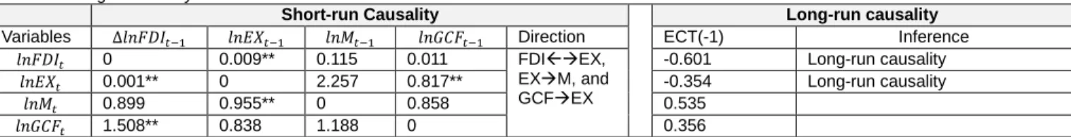
3.4. Granger-Casualty Test
In order to ascertain directional causality both in the short-run and in the long run, in study performs Granger- casualty test under error correction term. The causality among variables can be examined by using the following equation, where each variable treated as a dependent variable.
[
∆𝑙𝑛𝐹𝐷𝐼𝑡
∆𝑙𝑛𝐸𝑋𝑡
∆𝑙𝑛𝑀𝑡
∆𝑙𝑛𝐺𝑡
] = [ 𝛼11
𝛼21
𝛼31 𝛼41
] + [
𝑙𝑛𝐹𝐷𝐼𝑡−1
𝑙𝑛𝐸𝑋𝑡−1
𝑙𝑛𝑀𝑡−1 𝑙𝑛𝐺𝑡−1
] [ 𝛽11
𝛽21
𝛽31 𝛽41
𝛽12
𝛽22
𝛽32 𝛽42
𝛽13
𝛽23
𝛽33 𝛽43
𝛽14
𝛽24
𝛽34 𝛽44
] + ∑ [ 𝛾11
𝛾21
𝛾31 𝛾41
𝛾12
𝛾22
𝛾32 𝛾42
𝛾13
𝛾23
𝛾33 𝛾43
𝛾14
𝛾24
𝛾34 𝛾44
𝑞 ]
𝑠=1 [
∆𝑙𝑛𝐹𝐷𝐼𝑡−𝑠
∆𝑙𝑛𝐸𝑋𝑡−𝑠
∆𝑙𝑛𝑀𝑡−𝑠
∆𝑙𝑛𝐺𝑡−𝑠
] + [ 𝜗1 𝜗2
𝜃3
𝜗4
] 𝐸𝐶𝑇𝑡+ [ 𝜑1𝑡
𝜑2𝑡
𝜑3𝑡 𝜑4𝑡
] (11)
4. Results
4.1. Unit Root Test
While investigating long-run cointegration through
ARDL approach, determination of variables’ order of integration is not essential. Empirical studies, however, including Ouattara (2006), suggest the presence of second- order cointegration invalid estimated F-statistic for evaluation. To confirm the nonexistence of second-order integration of any variables, we purposively use ADF unit root test proposed by Dickey and Fuller (1979), P-P unit root
test proposed by Phillips and Perron (1988), and KPSS unit root test proposed by Kwiatkowski, Phillips, Schmidt, and Shin (1992). Unit root estimation reports in Table 3. The stationary test confirms none of the research variables are
integrated after the second difference, which induces us to move further for symmetric and asymmetric estimation between FDI and exchange rate.
Table 2: Unit root test estimation
ADF P-P KPSS
At level ∆ I At level ∆ I At level ∆ I
Bangladesh
lnFDI -3.69** - I(0) -3.69** - I(0) 0.11 0.35** I(1)
lnEX - 2.17 -4.15** I(1) -3.41 -4.01*** I(1) 0.12 0.27** I(1)
lnG -2.39 -3.98** I(1) -1.98* -4.60*** I(1) 0.09 0.22** I(1)
lnM -3.46 -5.26*** I(1) -6.51*** - I(0) 0.10 0.18** I(1)
Note 1. FDI for Foreign Direct Investment, EX for Exchange rate against US $, G for Gross Capital Formation, and M for money supply in the economy (M3).
Note 2. ∆ denotes first difference operator, I for an order of integration.
Note 3. ADF for augmented Dickey-Fuller test, P-P for Phillip–Perron and KPSS for Kwiatkowski–Phillips– Schmidt–Shin test Note 4. ***/** indicate significance at 1% and 5% levels, respectively.
4.2. Linear ARDL Estimation
In the previous section, we observed that variables show the different order of integration, under this situation best cointegration test can be performed using ARDL bound testing. In this section, we proceed to estimate ARDL
estimation based on symmetric effect assumption between exchange rate and FDI inflows applying linear ARDL bound testing approach proposed by Pesaran et al. (2001) and Narayan and Narayan (2005) by following pre-specified model equation (3a to 3d). Table 3 reports full information of estimation with four (04) Panel output.
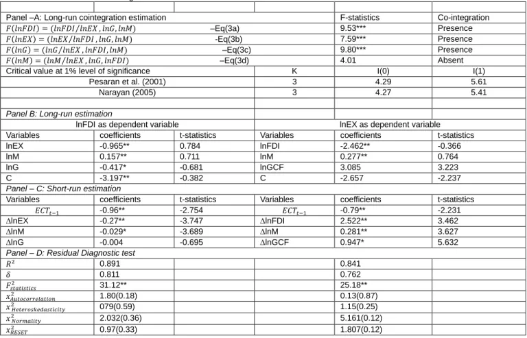
Table 3: Linear ARDL Bound testing
Panel –A: Long-run cointegration estimation F-statistics Co-integration
𝐹(𝑙𝑛𝐹𝐷𝐼) = (𝑙𝑛𝐹𝐷𝐼 𝑙𝑛𝐸𝑋⁄ , 𝑙𝑛𝐺, 𝑙𝑛𝑀) –Eq(3a) 9.53*** Presence 𝐹(𝑙𝑛𝐸𝑋) = (𝑙𝑛𝐸𝑋 𝑙𝑛𝐹𝐷𝐼⁄ , 𝑙𝑛𝐺, 𝑙𝑛𝑀) -Eq(3b) 7.59*** Presence 𝐹(𝑙𝑛𝐺) = (𝑙𝑛𝐺 𝑙𝑛𝐸𝑋⁄ , 𝑙𝑛𝐹𝐷𝐼, 𝑙𝑛𝑀) –Eq(3c) 9.80*** Presence 𝐹(𝑙𝑛𝑀) = (𝑙𝑛𝑀 𝑙𝑛𝐸𝑋⁄ , 𝑙𝑛𝐺, 𝑙𝑛𝐹𝐷𝐼) –Eq(3d) 4.01 Absent
Critical value at 1% level of significance K I(0) I(1)
Pesaran et al. (2001) 3 4.29 5.61
Narayan (2005) 3 4.27 5.41
Panel B: Long-run estimation
lnFDI as dependent variable lnEX as dependent variable
Variables coefficients t-statistics Variables coefficients t-statistics
lnEX -0.965** 0.784 lnFDI -2.462** -0.366
lnM 0.157** 0.711 lnM 0.277** 0.764
lnG -0.417* -0.681 lnGCF 3.085 3.223
C -3.197** -0.382 C -2.657 -2.237
Panel – C: Short-run estimation
Variables coefficients t-statistics Variables coefficients t-statistics
𝐸𝐶𝑇𝑡−1 -0.96** -2.754 𝐸𝐶𝑇𝑡−1 -0.79** -2.231
∆lnEX -0.27** -3.747 ∆lnFDI 2.522** 3.462
∆lnM -0.029* -3.689 ∆lnM 0.281** 3.627
∆lnG -0.004 -0.695 ∆lnGCF 0.947* 5.632
Panel – D: Residual Diagnostic test
𝑅2 0.891 0.841
𝛿 0.811 0.762
𝐹𝑠𝑡𝑎𝑡𝑖𝑠𝑡𝑖𝑐𝑠 2 31.12** 25.18**
𝑥𝐴𝑢𝑡𝑜𝑐𝑜𝑟𝑟𝑒𝑙𝑎𝑡𝑖𝑜𝑛 2 1.80(0.18) 0.13(0.87)
𝑥 𝐻𝑒𝑡𝑒𝑟𝑜𝑠𝑘𝑒𝑑𝑎𝑠𝑡𝑖𝑐𝑖𝑡𝑦 2 079(0.59) 1.15(0.25)
𝑥 𝑁𝑜𝑟𝑚𝑎𝑙𝑖𝑡𝑦2 2.032(0.36) 5.161(0.12)
𝑥𝑅𝐸𝑆𝐸𝑇 2 0.97(0.33) 1.807(0.12)
Table 3 (panel – A) reports F-statistics of various ARDL estimation along with the two critical value extracted from Pesaran et al. (2001) as well as Narayan (2005) which are quoted for small samples by following Bildirici and Ozaksoy (2017). It is observed from ARDL bound testing where each variable serves as the dependent variable in the equation. The study found F-statistics when FDI, EX, and M considered as dependent variables [ 𝐹(𝑙𝑛𝐹𝐷𝐼) = (𝑙𝑛𝐹𝐷𝐼 𝑙𝑛𝐸𝑋⁄ , 𝑙𝑛𝐺, 𝑙𝑛𝑀) = 9.53] , 𝐹(𝑙𝑛𝐸𝑋) = (𝑙𝑛𝐸𝑋 𝑙𝑛𝐹𝐷𝐼⁄ , 𝑙𝑛𝐺, 𝑙𝑛𝑀) = 7.53 , and 𝐹(𝑙𝑛𝐺) = (𝑙𝑛𝐺 𝑙𝑛𝐸𝑋⁄ , 𝑙𝑛𝐹𝐷𝐼, 𝑙𝑛𝑀) = 9.80 are higher than the upper bound of critical value at 1% level of significance (PCV = 5.61 and NCV=5.41). This is suggesting that the null hypothesis that is “no cointegration” cannot be accepted; rather we accept the existence of long-run cointegration between exchange rate, FDI inflows, monetary policy, and fiscal policy of Bangladesh. In particular, Study findings suggest exchange rate movement and FDI flows move together, which is supported by empirical studies by Lily et al. (2014).
Table 3 (Panel –B) reports long-run estimation for both models, where FDI and exchange rate serves as dependent variables in their respective equations. When FDI is treated as the dependent variable, the study found that the real exchange rate against the USD positively influences the FDI inflows in Bangladesh in the long run. It is implying that the real depreciation of the exchange rate boost inflows of FDI.
Findings are supported by empirical studied such as Froot and Stein (1991), Dees (1998), and Ang (2008).
Table 3 (Panel – C) exhibits short-run estimation. The short-run association specify the lagged error correction term 𝐸𝐶𝑇𝑡−1. We found the error correction term is negative and statistically significant (at 1%) in both cases, which confirm the existence of a short-run relationship between exchange rate and FDI inflows. The coefficients of both model (𝐸𝐶𝑇𝑡−1𝐸𝑋= −0.96, 𝐸𝐶𝑇𝑡−1𝐹𝐷𝐼= −0.79) indicate the high speed of adjustment towards long-run equilibrium with prior year shock in the exchange rate and FDI.
We also perform four residual diagnostic tests, see Table 3 (Panel – D), to confirm model construct validation and robustness in estimation as suggested by Pesaran et al.
(2001). Test of autocorrelation confirms that the estimated model is free from serial correlation, and test of normality ensure a normal distribution of error terms in the equation.
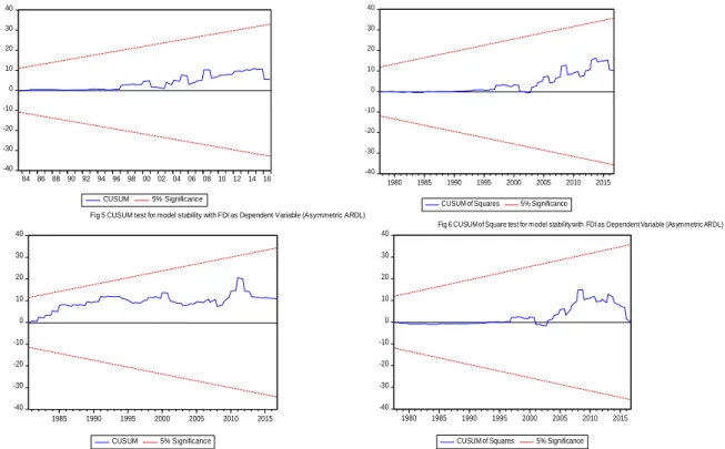
We also observed that the statistics of Ramsey’s RESET test confirm the correctness of model specification. Finally, to ensure estimation of long-run and short-run coefficient stability, by following Pesaran et al. (2001), we perform residual-based CUSUM and CUSUMSQ test, confirming that the estimating parameters are stable as lines between critical boundaries at a 5% level of significant (see Figure 1).
Figure 1: Residual-based CUSUM and CUSUMSQ test
-40 -30 -20 -10 0 10 20 30 40
1980 1985 1990 1995 2000 2005 2010 2015
CUSUM 5% Significance
Fig 3 CUSUM test for model stability with Exchang rate as Dependent Variable -40 -30 -20 -10 0 10 20 30 40
1980 1985 1990 1995 2000 2005 2010 2015
CUSUM of Squares 5% Significance
Fig 4 CUSUM of Square test from model stabiity with exchange rate as Dependent Variable -40
-30 -20 -10 0 10 20 30 40
1980 1985 1990 1995 2000 2005 2010 2015
CUSUM of Square 5% Significance
Fig 2 CUSUM of Square test for model stability with FDI as Depented Variable -40
-30 -20 -10 0 10 20 30 40
1980 1985 1990 1995 2000 2005 2010 2015
CUSUM 5% Significance
Fig 1 CUSUM test for Model stability with FDI as Dependent Variable
4.3. Nonlinearity Estimation for the Period 1974Q1-2016Q4
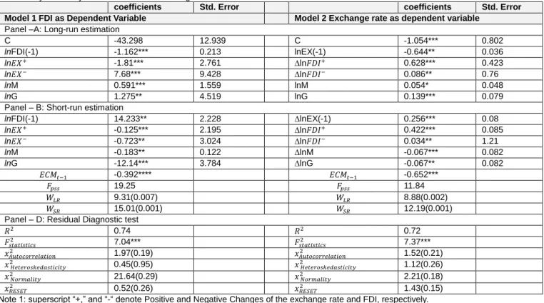
The previous section provides evidence of a linear relationship between the exchange rate and the inflows of FDI. Findings are consistent with theoretical and empirical studies. Now, we move towards examining the existence of asymmetric relationship by applying newly nonlinear ARDL approach proposed by Shin et al. (2014) following model (9) and (10). Table 4 reports full information on asymmetric estimation. To ascertain robustness and stability in the model estimation, we performed several residual-based
diagnostics tests see, Table 4 (panel-D), as suggested by empirical studies. It is seen from a residual test, that model is free from serial correlation, error terms normally distributed and no problem of homoscedasticity. Moreover, The Ramsey’s RESET confirms model construction validity as well. Model estimation stability investigated by applying residual recursive test proposed by Pesaran et al. (2001), commonly known as CUSUM and CUSUM of the square, ascertaining the model stability in estimation as the parameters fall within the critical value at a 5% level of significance (Figure 2).
Figure 2: CUSUM and CUSUM of the square Now we proceed to estimate the existence of
cointegration test, in particular, joint cointegration test in both nonlinear equation 9 and 10. We found test statistics of 𝐹(𝑓𝑑𝑖)𝑝𝑠𝑠= 19.25 and 𝐹(𝑒𝑥)𝑝𝑠𝑠= 11.84 is higher than the upper bound of critical value14 at 1% level of significance. So we can conclude in favor of asymmetric long-run association between examined variables. It is also observed that the coefficients’ error correction term (𝐸𝐶𝑇𝑡−1) in case of both tested model is negative and statistically significant at 1% level of significance. It supports the previous confirmation of long run co- integration. The coefficients of error correction term -0.39 in case of FDI as the dependent variable and -0.625 in case of
4 Following Shin et al. (2011), we adopted a conservative approach to the choice of critical values and employed k = 1.
the exchange rate as the dependent variable in the model estimation, which is negative and statistically significant at a 1% level of significance. The error correction term explained that any shock in the short run could be absorbed and reach the long run equilibrium at a speed of 39% and 62%
per quarter.
We performed a standard Wald test to investigate the symmetric relationship. In Table 4 (panel –C), 𝑊𝐿𝑅 indicates a Wald test with null hypothesis symmetric relationship (𝐿+𝐸𝑋 =𝐿𝐸𝑋− and 𝐿+𝐹𝐷𝐼 =𝐿−𝐹𝐷𝐼). The null hypothesis of the short-run symmetric relation 𝑊𝑆𝑅 (𝑆𝐸𝑋+
=𝑆𝐸𝑋− and 𝑆𝐹𝐷𝐼+ =𝑆𝐹𝐷𝐼− ). For the long run, the null hypothesis of symmetric relation is rejected at 1% level of significance. More particularly, we found 𝑊𝐿𝑅(𝑓𝑑𝑖)= 9.312(𝑝 − 0.0079) of model (9), and 𝑊𝐿𝑅(𝑓𝑑𝑖)= 8.88(𝑝 − 0.0025) for the model (10). For the short-run
-40 -30 -20 -10 0 10 20 30 40
84 86 88 90 92 94 96 98 00 02 04 06 08 10 12 14 16
CUSUM 5% Significance
Fig 5 CUSUM test for model stability with FDI as Dependent Variable (Asymmetric ARDL) -40 -30 -20 -10 0 10 20 30 40
1980 1985 1990 1995 2000 2005 2010 2015
CUSUM of Squares 5% Significance
Fig 6 CUSUM of Square test for model stability with FDI as Dependent Variable (Asymmetric ARDL)
-40 -30 -20 -10 0 10 20 30 40
1985 1990 1995 2000 2005 2010 2015
CUSUM 5% Significance
Fig 7 CUSUM test for model stability with Exchange rate as Dependent variable (Asymmetric ARDL) -40 -30 -20 -10 0 10 20 30 40
1980 1985 1990 1995 2000 2005 2010 2015 CUSUM of Squares 5% Significance
Fig 8 CUSUM of Square test for model stability with Exchange rate as Dependent Variable (Asymmetric ARDL)