Acoustic characteristics of Anchovy schools, and visualization of their connection with water temperature and salinity in the Southwestern Sea and the Westsouthern Sea of South Korea

서 론

지난 수십년 동안 수산 음향학에 관련한 하드웨어와 소프트웨어의 개발과 발전은 효율적이면서 생태계에

큰 영향없이 수중 생물양을 평가할 수 있게 하였고, 어 류 행동의 모니터링과 분포 패턴에 관한 보다 정도 높은 정보를 제공해주었다. 특히 과학어군탐지기를 이용하

서해 남부와 남해 서부의 한 정점에서 수온 및 염분과 멸치 어군의 특징의 관련성 시각화

강명희·최석관¹*·황보규²

경상대학교 해양경찰시스템학과, 해양산업연구소, ¹국립수산과학원 자원관리과,

2군산대학교 해양생산학과

Acoustic characteristics of Anchovy schools, and visualization of their connection with water temperature and salinity in the Southwestern

Sea and the Westsouthern Sea of South Korea.

Myounghee K ANG , Seok-Gwan C HOI

*, and Bo-kyu H WANG

Department of Maritime Police and Production System, The institute of Maritime Industry, Gyeongsang National University, Tongyeong 650-160, Korea

1

Fisheries Resources Management Division, National Fisheries Research & Development Institute, Busan 619-705, Korea

2

Department of Marine Science and Production, Kunsan National University, Kunsan, 573-701, Korea

Morphological and positional characteristics of anchovy aggregations, confirmed by trawling, were examined in two locations of the southern part of the West Sea (T1) and the western side of South Sea (T11) of South Korea. Morphological characteristics (mean length, height and area) of the anchovy aggregations at T1 were smaller than those at T11, however the positional char- acteristics (distributional depth and bottom depth) of the aggregations at T1 were larger than those at T11. Diverse dataset such as the ship’scruise track, the cruse map, and interpolated three-dimensional-like water temperature were visualized in multiple dimensions. For a comprehensive understanding of the anchovy aggregations within their surrounding circumstances, the inter- polated water temperature transferred to the location of anchovy aggregations at both stations were visualized based on geospatial information. Using quantitative investigation, the overall range of change in water temperature and salinity of anchovy aggre- gations at stations was considerably small. However, the water temperature and salinity of anchovy aggregations at T11 were somewhat higher than those at T1.

Keywords : Anchovy, Acoustic, Morphological, Positional, Visualization

http://dx.doi.org/10.3796/KSFT.2014.50.1.039

*Corresponding author: [email protected], Tel: 82-51-720-2323, Fax: 82-51-720-2337

< Original Article>

는 수중 음향 기술은 해양뿐만이 아니라 담수환경에서 도 고분해능의 데이터를 수집할 수 있어 다양한 수중 생 물종의 밀도 분포와 행동 연구를 위한 중요한 수단으로 이용되고 있다 (Simmonds and Maclennan, 2005).

멸치는 극지방과 열대지역을 제외한 온대 기후를 가 지는 나라에서 대부분의 연안역에 분포하고 있다. 또한 멸치는 플랑크톤을 섭취하면서 다른 어종의 먹이로써 중요한 역할을 하고 있다. 따라서 멸치는 연안해역에서 생태계의 먹이 사슬을 유지하는데 매우 중요한 비중을 차지한다 (Shelton et al., 1993). 게다가 세계 여러 나라의 연안 해역에서 매년 많은 양의 멸치가 어획되고 있어 상 업적으로도 중요한 어종이라 할 수 있다. 이러한 이유로 세계의 여러 해역에서 수중 음향 기술을 이용하여 멸치 어군의 공간적인 패턴, 분포 및 행동, 생물량의 추정에 관한 조사가 활발히 이루어지고 있다. 예를 들면, 1983 년부터 약 167 km에 달하는 페루 연안을 따라서 멸치 (Engraulis ringens) 음향 조사가 수행되어 왔고, 그 자원 량은1987년부터 2002까지는 2백만톤에서 천만톤으로 추정되었다 (Gutierrez et al., 2007). 또한 페루 Humboldt 해류에 의해 멸치 어군의 집합 패턴과 그 변동이 크게 좌우된다고 밝혔다. 남아메리카에서는 1984년 이후로 음향 조사를 이용하여 멸치 (Engraulis encrasicolus) 어 군의 자원량과 공간적인 분포 특징을 조사해왔다 (De- moor et al., 2008). 중국의 황해에서는 1984년부터 2002 년까지 멸치 (Engraulis japonicus)의 겨울철 자원량은 음 향학적으로 추정하여 매년 어획되는 양과 비교 연구한 사례가 있다 (Zhang et al., 2011). 1990년 중반 이전까지 이 해역에서 멸치 자원량은 약 2〜3백만톤으로 추정되 었으며, 1996년에서 1998년 사이에는 자원량의 갑작스 런 하락을 보였다. 또한 같은 해역을 대상으로 멸치의 in

situ

graulis japonicus)

Amakasu et al., 2010). 1990년후반 이후로 남해안, 황해, 일본 주변의 태평양 서북해역을 대상으로 멸치의 공간 적 인 패 턴 과 생 물 량 의 추 정 을 보 고 한 바 가 있 다 (Ohshimo, 1996; Ohshimo, 2004; Murase et al., 2009;

Murase et al., 2012). 우리나라에서도 멸치 (Engraulis

japonicus)는 생태학적으로도 상업적으로도 매우 중요

2000년과 2001년에는 보다 넓은 남해안 해역에 분포하 는 멸치어군을 대상으로 자원량을 추정한 바가 있다 (Choi et al., 2001). 또한 120 kHz에서 멸치 측면의 in situ TS (Lee and Kang, 2010)와 38, 120, 200 kHz에서 ex situ TS를 측정한 바가 있다 (Kang et al., 2009). 2008년과 2009 년에는 통영 주변의 멸치 현존량을 추정한 사례가 있다 (Kim et al., 2008; Oh et al., 2009).

앞서 언급한 많은 연구사례를 통해 멸치는 해양 환경 에 따른 어군의 공간적 분포와 형태가 변화함을 알 수 있다. 따라서 멸치 어군의 다양한 특징, 예를 들어 형태 학 및 위치학적인 특징을 파악하는 것과, 해양 환경을 고려한 이들의 특징을 이해하는 것은 매우 중요하다. 제 주도 해역에서 해양 환경 (수온, 염분, 용존산소, 클로로 필a, 부유물질 등)에 따른 멸치 치자어의 분포와 수온 전 선에 따른 남해 및 서해 연안역에서 멸치난치어의 분포 를 연구한 사례가 있다 (Kim, 1983; Ko et al., 2007). 이 외 에도 해양 환경과 멸치 어군에 관한 연구 사례의 결과를 다차원으로 가시화할 수 있다면, 해양 환경에 근거한 멸 치 어군에 관한 보다 포괄적인 생태 및 분포 특징을 이해 하는데 유용하게 쓰일 수 있다고 생각한다. 따라서 본 연 구의 목적은 서해 남부와 남해 서부에 분포하고 있는 멸 치 어군의 형태학 및 위치학적인 특징을 살펴보며, 이 어 군과 해양환경 즉, 수온과 염분과의 관계를 알아보고 시 각화하고자 한다. 중장기적으로 이 연구는 멸치 어군의 밀도와 다양한 특징과 해양 환경과의 관계를 시각화하 고 정량적으로 조사하기 위한 기초 연구라고 할 수 있다.

재료 및 방법

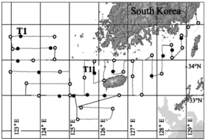
수중 음향 조사, 보다 구체적으로 트랜젝트 라인 음향 조사는 트롤 조사와 함께 2003년 3월 19일에서 4월 10일 까지 남해안과 서해 남부 해역에서 실시되었다 (Fig. 1).

조사선은 국립수산과학원 탐구 1호 (2150톤)를 이용하 였고, 38과 120kHz가 설비된 EK500과학어군탐지기 (Simrad)를 사용하였다. 조사 첫날에는 표준 교정 절차 에 따라서 과학어군탐지기를 교정하였다 (Foote et al., 1987). 조사선의 속도는 조사 기간 동안 약 10knots를 유 지하였다. 생물학적인 샘플링을 위해서 중층 트롤네트 를 사용하였고, 트롤네트의 길이는 70m이고, 평균 예망 속도는3.6 knots, 평균 예망 시간은 32.4분이었다. 트롤 조업은 낮 동안만 16회 수행하였다. 트롤의 위치는 어군 탐지기의 에코그램에서 어군같은 신호가 출현한 것을 토대로 결정하였다. 각 트롤 정점에서 얻은 표본은 우선 적으로 어종을 식별하고 체중과 체장을 선상에서 측정 하였다. 해양 환경 테이터를 수집하기 위해서 수온염분 수심기록계 (Conductivity Temperature Depth, CTD이하,

SBE 911, Sea-Bird)를 사용하였고, CTD인양속도는 1m/s 이였다. CTD 정점은 총36개이며, 가능하면 음향조사의 한 개의 트랜젝트 라인 양쪽 끝과 중앙에 정점을 선정하 여 라인별 3정점에서 해양 환경 데이터를 수집하려고 하였다.

과학어군탐지기의 음향데이터는 에코뷰 (Echoview ver. 5.3, Myriax)에 직접 입력하여 분석하였다. 멸치 어 군의 형태학 및 위치학적인 특징을 이해하기 위해서, SHAPES 어군 탐지 알고리즘 (Barange, 1994)을 이용하 여 어군을 다각형으로 정의하고 그 다각형의 형태학 및 위치학적인 특징, 즉 형태학적 및 위치학적인 정보를 추 출하였다. 어군 탐지 알고리즘은 38 kHz 에코그램에서 적용하고 이때 사용한 파라메터는 Table 1과 같다.

일반적으로 멸치 어군은 낮 동안에는 작은 사이즈로 도 분포한다고 알려져 있으므로 (Fujino et al., 2010), 작 은 사이즈의 어군이라 할지라도 탐지될 수 있도록 파라 메터를 선정하였다. 트롤 조사로 어획된 어종 중에 멸치 로 확인된 트롤 정점에서만 이 어군탐지를 실시하였다.

이 어군 탐지 알고리즘을 적용하기 전에, 트롤 정점 1 주 변에 약 5〜10m의 불연속적인 얇은 띠가 발견되어 이것 은 데이터 분석에서 제외시켰다. 탐지된 어군의 형태학 및 위치학적인 특징을 설명하는 기술어는 콤마분류저 장방식 (Comma Separated Values, CSV)형식으로 변환하 였다. 어군탐지기는 GPS의 신호를 받아서 위치 정보 (위도와 경도)를 파악하므로 음향 데이터는 GPS 신호를 포함하고 있다. 음향 데이터에 내재되어 있는 GPS 데이 터를 이용하여 항적선을 작성할 수 있으며, 이 데이터를 조사 해역에서 멸치 어군과 주변 환경과의 관계를 가시 화하는데 사용하기 위해서 CSV형식으로 변환하였다.

마지막으로 에코뷰에서 자동적으로 생성되는 항적도는 포트블 네트워크 그래픽스 (Portable Network Graphics, PNG)형식으로 변환하였다.

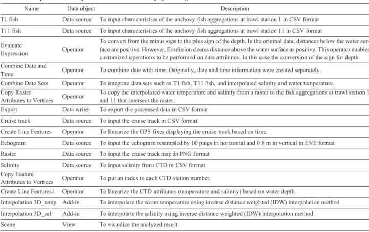
멸치 어군과 해양 환경과의 관계를 이해하고 가시화 하기 위해서 이온퓨전 (Eonfusion ver. 2.5, Myriax)을 이 용하여 작성한 데이터 플로는 Fig. 2에 표시하였다. 데이 터 플로에서 정칠각형으로 표시된 오브젝트의 상세한 설명은 Table 2에 기재하였다. 이 데이터 플로에서 탐지 된 어군의 공간 위치와 보간된 해양 환경 데이터의 위치 가 같을 경우, 해양 환경 데이터의 속성 (수온과 염분)은 어군의 데이터로 옮겨진다. 즉, 이들 데이터가 공간적으 로 동일한 위치일때 해양 환경 데이터의 속성과 어군의

Table 1. The parameter settings for detecting fish schools at 38 kHz

Fig. 1. Map of the study area. The line indicates the ship’s cruise track, the closed circle refers to the trawl station, and the open circle represents the CTD probe station. T1 refers to the trawl station 1 and T11 means trawl station 11.

Setting parameter Value

Minimum data threshold Minimum total school length Minimum total school height Minimum candidate length Minimum candidate height Maximum vertical linking distance Maximum horizontal linking distance

−70 dB

3 m

1 m

3 m

1 m

3 m

7 m

Fig. 2. Dataflow of geospatial analysis. Objects in light gray color are data sources, and objects in dark gray are final results which are “scene”

for visualization and “export” for exporting analyzed results. Dataflow reflects the logical flow and transformation of information from data sources (light gray) via a series of operator objects (white color) to the scene and to export (dark gray). A set of objects can be connected though pipes. Each object has its property which controls its functionality. A description of each object is described with precision in Table 2.

Table 2. Description of each object in dataflow which is displayed in Fig. 2

Name Data object Description

T1 fish Data source To input characteristics of the anchovy fish aggregations at trawl station 1 in CSV format T11 fish Data source To input characteristics of the anchovy fish aggregations at trawl station 11 in CSV format Evaluate

Expression Operator

To convert from the minus sign to the plus sign of the depth. In the original data, distances below the water sur- face are positive. However, Eonfusion deems distance above the water surface as positive. This operator enables customized operations to be performed on data attributes. In this case the conversion of the sign for depth.

Combine Date and

Time Operator To combine date with time. Originally, date and time information were created separately.

Combine Date Sets Operator To integrate data sets such as T1 fish, T11 fish, and interpolated salinity and water temperature.

Copy Raster

Attributes to Vertices Operator To copy the interpolated water temperature and salinity from a raster to the fish aggregations at trawl station 1 and 11 that intersect the raster.

Export Data writer To export the processed data in CSV format Cruise track Data source To input the cruise track in CSV format

Create Line Features Operator To linearize the GPS fixes displaying the cruise track based on time.

Echogram Data source To input the echogram resampled by 10 pings in horizontal and 0.8 m in vertical in EVE format Raster Data source To input the cruise track map in PNG format

Salinity Data source To input salinity from CTD in CSV format Copy Feature

Attributes to Vertices Operator To put an index to each CTD station number.

Create Line Features1 Operator To linearize the CTD attributes (temperature and salinity) based on water depth.

Interpolation 3D_temp Add-in To interpolate the water temperature using inverse distance weighted (IDW) interpolation method Interpolation 3D_sal Add-in To interpolate the salinity using inverse distance weighted (IDW) interpolation method

Scene View To visualize the analyzed result

특징 (속성이라고 할 수 있음)은 서로 이동될 수 있으므 로 이들 데이터간의 관계를 비교, 조사할 수 있다. 그리 고 역거리가중법 이용하여 해양 환경 데이터를 보간하 여 여러 층으로 만들어 3차원적으로 가시화하였다. 여 기서, 역거리가중법은 가까이 있는 실측값에 더 큰 가중 치를 주어 보간하는 방법 (Tomczak, 1998)으로, Kang et al. (2011)에 상세하게 서술하였다. 마지막으로 동일한 위치 정보를 근거로 탐지된 어군과 보간된 해양환경 데 이터를 짝으로 하여 CSV형식으로 변환하였다.

결 과 트롤 어획 결과

트롤 정점별로 어획된 어종에서 가장 많이 어획된 어

종, 두번째와 세번째로 많이 어획된 어종을 Table 3에 나 타내었다. 트롤 정점 1에서 멸치가 어획된 비율은 91%, 정점 11에서 어획된 멸치 어군의 비율은 94%이었다. 즉 이 두 트롤 정점에서 멸치 어군이 거의 단일 어종으로 분포한다고 간주할 수 있다. 따라서 이 두 트롤 정점에 서의 멸치 어군을 대상으로 어군의 특징과 해양 환경과 의 관계를 시각화한다. 이 두 정점에서 어획된 멸치의 평균 체장은 정점 1에서는 10.7±1.3cm, 정점 11에서는 9.9±1.5cm이었다.

멸치 어군의 형태학 및 위치학적인 특징

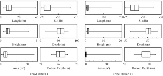
멸치 어군의 형태학 및 위치학적인 특징을 Fig. 3에 나 타내었다. 트롤 정점 1과 11에서 멸치 어군의 75% 는 어

Table 3. The most caught species and its percentage, the second most caught species and its percentage, and the third caught species and its percentage by each trawl station

Trawl St. The most occupied species Percent (%)

The second most occupied species

Percent (%)

The third most occupied species

Percent (%)

1 Anchovy

(Engraulis japonicus) 91 Leptocephalus

(Congridae) 3.7 Korean pomfret

(Pampus echinogaster) 2.7

2 Anchovy

(Engraulis japonicus) 51 Hairtail

(Trichiurus lepturus) 23 common hairfin anchovy

(Setipinna tenuifilis) 7.4

3 Anchovy

(Engraulis japonicus) 69 Hairtail

(Trichiurus lepturus) 24 Korean pomfret

(Pampus echinogaster) 6.3

4 Anchovy

(Engraulis japonicus) 16 Hairtail

(Trichiurus lepturus) 33 Yellow goosefish

(Lophius litulon) 13

5 Yellow croaker

(Larimichthys polyactis) 30 Hairtail

(Trichiurus lepturus) 27 Yellow croaker

(Larimichthys polyactis) 8.5

6 Hairtail

(Trichiurus lepturus) 24 Yellow croaker

(Larimichthys polyactis) 22 Conger eel

(Conger myriaster) 19

7 Yellow croaker

(Larimichthys polyactis) 35 Korean pomfret

(Pampus echinogaster) 25 Brown croaker

(Miichthys miiuy) 10.2

8 Yellow goosefish

(Lophius litulon) 24 Crustacean

(Lophiomus setigerus) 18.6 Anger fish

(Champsodon snyderi) 10.8

9 Hairtail

(Trichiurus lepturus) 48 Yellow goosefish

(Lophius litulon) 27 Japanese spanish marckerel

(Scomberomorus niphrnius) 10.3

10 Lantern fish

(Benthosema pterotum) 56 Yellow croaker

(Larimichthys polyactis) 10.5 Anger fish

(Lophiomus setigerus) 9

11 Anchovy

(Engraulis japonicus) 94 Japanese mackerel

(Scomber japonicas) 2.4 Rock fish

(Sebastes schlegeli) 1.4 12 Blackmouth angler

(Lophiomus setigerus) 22 Japanese spanish mackerel

(Scomberomorus niphrnius) 14 White croaker

(Argyrosomus argentatus) 9.2 13 Japanese flying squid

(Loligo japonicas) 20 Surinam Squid

(Todarodes pacificus) 20 Japanese spanish mackerel

(Scomberomorus niphrnius) 8.1

14 Korean pomfret

(Pampus echinogaster) 30 Yellow goosefish

(Lophius litulon) 27 Crab

(Portunus trituberculatus) 4

15 Hairtail

(Trichiurus lepturus) 62 Korean pomfret

(Pampus echinogaster) 22 Anger fish

(Lophiomus setigerus) 5.9

16 Korean pomfret

(Pampus echinogaster) 56 Hairtail

(Trichiurus lepturus) 15.3 Yellow goosefish

(Lophius litulon) 9.8

군의 길이, 높이와 면적이 작은 사이즈로 구성되어 있음 을 알 수 있다. 그러나, 트롤 정점 1에서 멸치 어군의 평 균 깊이, 높이, 면적은 각각 9.7m, 1m, 10.3m²이었고, 트 롤 정점 11에서의 멸치 사이즈는 정점 1보다 약간 큰 15.1m, 1.8m, 31.9 m²이었다. 트롤 정점 1에서의 멸치 어 군의 50% (일사분위수〜삼사분위수)는 –65.6〜–

58.7dB의 SV범위를 가지고, 분포 수심의 범위는 46.5〜

65.3m, 해저 수심은 75.7〜76.7m의 범위를 보였다. 특히 트롤 정점 1에서 멸치 어군의 해저 수심은 75〜77m로 거의 일정함을 보였다. 트롤 11에서 멸치 어군의 50%는 SV(－63.5〜－54.5dB), 분포 수심 (46.7〜57.2 m), 해저 수심 (64.1〜70.9m)을 보였다. 따라서 트롤 정점1에서의 멸치 어군의 형태학적인 특징은 트롤 정점 11보다는 작 다고 할 수 있다. 그러나 위치학적인 특징을 살펴보면, 정점 1에서의 멸치 어군의 분포 수심과 해저 수심은 정 점 11의 것보다 더 크다고 할 수 있다.

멸치 어군과 해양 환경 데이터간의 관련성과 시각화 멸치 어군과 주변 해양 환경 데이터를 다차원적으로 시각화하여, 중장기적으로 해양 환경을 근거로 하는 멸 치 어군에 관한 포괄적인 생태 및 분포적 특징과 밀도 평가를 수행하기 위한 기초 자료로 활용할 수 있다. 다 차원적 가시화의 의미는 3차원 즉 위도, 경도, 수심뿐만 이 아니라 시간 혹은 어떤 다른 데이터의 속성을 포함시 키는 것을 말한다. 예를 들어 수심 정보를 중심으로 변

환한 조사선의 항적선, 항적도, 보간한 3차원적인 수온, CTD정점의 위치 데이터를 이용하여 Fig. 4과 같이 시각 화하였다. 남해 서부의 수온 범위는 12〜16.5 °C인데 비 해 서해 남부의 수온은 7.5〜9 °C의 범위를 가진다. 개략 적으로 말하면, 남해 서부의 남서쪽 해역을 중심으로 좌 우로 두 개의 다른 수온을 가진 수괴가 존재하는 것으로

Fig. 3. Boxplot of various characteristics of anchovy aggregations in trawl station 1 and 11. Half samples (boxes) and the first and third quartiles (bars) are shown. A logarithmic scale is used for Sv. Note that different scales were used in each trawl station.

Trawl station 1

0 20 40 -70 -50 -30

Length (m) S

(dB) Length (m) S

(dB)

Height (m) Depth (m) Height (m) Depth (m)

Area (m

) Bottom Depth (m) Area (m

) Bottom Depth (m)

0 5 0 50 100 0 10 20 50 50

0 50 74 76 78 0 500 50 70

0 100 200 -70 -50 -30

Trawl station 11

Fig. 4. Multi-dimensional visualization of diverse dataset such as the ship’s cruise track, the cruse map, interpolated three-dimensional- like water temperature, and CTD stations. The white triangle shows the location of trawl station 1, and the white circle indicates the trawl station 11. The cruise track is displayed in black transect line.

Many layers of the interpolated water temperature look like three dimensions. The slide bar on the bottom shows the water depth.

While the slider is moving from side to side, only the interpolated

water temperature relevant to the slide of water depth will be

shown. The multiple vertical lines inside interpolated water temper-

ature are CTD stations.

설명할 수 있다. 이 시각화 기능을 통하여, 조사 해역 전 체와 각 데이터 간의 관계를 이해하는데 도움을 줄 수 있다.

멸치 어군과 해양 환경데이터 사이의 관계를 가시화 하기 위해서, 환경 데이터 속성 즉 보간한 수온과 염분 을 지리 공간적으로 중첩하는 어군 데이터로 이동 변환 한 것을 이용하였다. 트롤 정점 1과 11에 탐지된 멸치 어 군의 평균S^V와 어군과 동일한 위치에서의 수온을 멸치 어군의 색깔로 표시하였다 (Fig. 5). 여기서 어군의 면적 은 구의 크기와 비례하므로 구가 클수록 어군의 면적이 큼을 알 수 있다. 트롤 정점 1과 11에서 수심 중간쯤에 상대적으로 다소 높은 SV값 (–55〜–43 dB)을 가진 어 군이 보이지만, 이 보다 높은 S^V범위 (–46〜 –43 dB)를 가진 어군은 트롤 정점 11에서만 존재함을 알 수 있다.

두 정점에서 다소 큰 사이즈의 어군은 보다 수심이 얕은 쪽에 위치하고 있다. 트롤 정점 1에서 멸치 어군의 수온

범위는 9.4〜9.8 °C이고, 트롤 정점 11에서 멸치 어군의 수온 범위는 11.2〜11.6 °C이다. 따라서, 트롤 11에서의 멸치 어군은 정점 1에서의 어군보다 약 2°C 높은 수온 에서 분포하는 것을 알 수 있다. 이와 같이 다차원의 시 각화는 수온과 같은 환경 데이터와 어군사이의 관계를 직접적으로 이해하기 위해서 유용하게 사용될 수 있다 고 생각한다. 또한 데이터간 상호 관계의 가시화뿐만이 아니라 그 관계를 직접적으로 표시할 수 있다.

앞서 설명한 동일한 위치 정보를 근거로 멸치 어군과 해양 환경 데이터를 한 짝으로 하고 CSV형식으로 변환 한 데이터를 이용하여, 트롤 정점1과 11에서 멸치 어군 이 분포하는 정확한 수온과 염분을 빈도분포로 표시하 였다 (Fig. 6). 트롤 정점 1에서 멸치 어군의 수온 범위는 8.6〜9.8°C이고, 평균 수온은 9.5 ± 0.3°C이다. 즉 멸치 어군의 대부분 (90%)은 9°C이상의 수온에서 분포한다.

트롤 정점 11에서 멸치 어군의 수온범위는10.8〜12°C

Fig. 5. Mean SV (dB re 1/m) of every anchovy aggregation in trawl station 1(a) and 11(b), and interpolated water temperature (°C) transferred to the location of all anchovy aggregations in trawl station 1(c) and 11(d). The green line above each panel represents the cruise track. The band in dark brown under the green line represents the ring down noise from the transducer. The dark brown near bottom shows the sea bottom. The SV color legend is used in (a) and (c). A sphere represents an anchovy aggregation detected. The size of a sphere is directly relates to the area (m3) of an anchovy aggregation. Note that the range of the area legends and temperature legends at trawl station 1 and 11 are dif- ferent.

(a)

(d) (c)

(b)

이며, 그 평균 수온은 11.3 ± 0.1°C이다. 즉 트롤 정점 11 에서 대부분의 어군은 11 °C이상의 수온에 분포하였으 며, 특히 멸치 어군의 47%는 수온 범위 11.2〜11.4 °C에 분포하였다. 한편, 트롤 정점 1에서 평균 염분은 33.3 ± 0.1 psu이고, 대부분의 멸치 어군 (83%)은 33.2〜33.4 psu 의 범위에 분포한다. 트롤 정점 11에서 멸치 어군의 평 균 염분은 33.9 ± 0.1 psu이고 대다수의 멸치 어군 (83%) 은 33.8〜33.9 psu 범위에 분포한다. 결론적으로 두 정점 에서 멸치 어군의 수온과 염분의 변화는 매우 적지만, 트롤 정점 11에서 멸치 어군의 수온과 염분은 정점 1보 다 다소 높다는 것을 알 수 있다.

고 찰

우리나라 동해안 남부해역에서 멸치 어군의 형태 및 분포 특징을 1996년에 조사한 사례가 있다 (Kang, 1996).

이 해역에서 분포하는 멸치의 평균 길이, 높이, 면적은 각 각 26m, 8m, 52m²이었고, 멸치 어군의 평균 S^V은 –37.2 dB이였다. 본 연구에서의 멸치 어군의 크기와 비교해보 면, 동해안의 멸치 어군이 두 배가량 큰 것을 알 수 있다.

1994년 3월에 동중국해에서, 1995년 3월말과 4월초에는 남해안의 동부해역에서 멸치의 형태학적인 특징을 계 측한 연구가 있다 (Kim et al., 1998). 동중국해에서 멸치 어군의 평균 길이, 높이, 면적은 각각 13.8m, 3.4m,

29.5m²이었고, 남해안 동부 해역에서는 각각 22.7m, 4.4m, 69.4m²으로 조사되었다. 지리학적으로 동중국해 는 본 연구에서 트롤 정점 1보다 정점 11에 더 가깝다.

이 연구의 동중국해에서 멸치 어군의 형태학적인 특징 은 본 연구의 트롤 정점 11에서의 어군 특징과 근사함을 알 수 있다. 두 연구에서의 분포 수심은 거의 동일하였 고, 이때 수심은 52m이었다. 그러나 이 연구에서 남해안 에서의 평균S^V는 –53.4 dB으로 트롤 정점 11 (–58.4 dB)보다는 다소 높은 것으로 보인다. Ohshimo et al.

(1996)는 본 연구와 거의 유사한 해역에서 멸치 어군 형 태의 유사성을 보여주었다. 이 연구에서 어군탐지기 FQ70 (50kHz, Furuno)을 이용하여 조사한 어군의 평균 길이와 높이는 각각 16.3m와 3.3m이었다. 한편 우리나 라 주변에서의 멸치는 일반적으로 계절에 따라 동중국 해로부터 남해안의 서쪽 해역에서 동쪽 해역으로 그리 고 동해안으로 이동하는 것으로 알려져 있다. 예를 들 면, 봄에는 동중국해에서 멸치는 쓰시마 난류를 따라 여 수, 남해, 통영으로 이동하는 것으로 알려져 있다. 6월이 되면 멸치는 동해안의 강원도 연안까지 이동하는 것으 로 보인다 (Park et al., 1996). 동중국해로부터 남해안과 동해안으로 이동하면서 멸치어류의 체장은 성장하며 이에 따라 멸치 어군을 이루는 분포 패턴은 변화할 것으 로 생각한다. 따라서 이러한 추론으로 말미암아 동해안

Fig. 6. Frequency distribution of interpolated water temperature and salinity transferred to the location of all anchovy aggregations when they were overlapping. Water temperature and salinity of all anchovy aggregations at trawl station 1 are (a) and (b) respectively, and those at trawl station 11 are (c) and (d).

(a) (c)

(b) (d)

60 40 20 0

8.6 － 8.8 8.8 －

9 9 －

9.2 9.2 － 9.4 9.4 －

9.6 9.6 － 9.8

32.8 －33 33 －33.2 33.2 －33.4 33.6 －33.8 33.8 －33.9 33.9 －34.1 Water temperature (。C)

Salinity (psu) 10.8 －

11 11 － 11.2 11.2 －

11.4 11.4 － 11.6 11.6 －

11.8 11.8 － 12

100

50

0

100

50

0

F re qu en cy (% )

60

40

20

0

의 멸치어군의 크기 (Kang, 1996)는 본 연구의 멸치 어군 보다 크다고 생각한다.

Choi et al. (2001)는 2000년과 2001년에 남해안의 멸치 를 대상으로 수중 음향 조사를 실시하면서 해양 환경 데 이터를 수집하였다. 두 해 동안 멸치 어군이 우세한 해 역은 남해안 동부해역이였으며, 이 해역에서의 수온 범 위는 12〜15°C이고, 염분 범위는 33.6〜34.5 psu이었다.

남해안 동부해역의 수온 (12〜15°C)과 본 연구의 남해 서부 해역의 수온 (8.6〜12°C)과 비교해 보면, 전자가 조 금 더 따뜻함을 알 수 있다. 하지만, 두 연구에서의 염분 은 유사한 것으로 보인다. 일반적으로 남해안 동부해역 의 수온은 서부해역보다 약간 따뜻한 것을 알 수 있다.

다양한 데이터 형식과 샘플링 크기를 가지는 데이터 상호간의 관계를 직접적으로 비교 파악하고 데이터를 종합적으로 가시화하는 방법은 수집한 데이터를 보다 포괄적으로 이해하면서 데이터간의 상호작용도 알 수 있는 장점이 있다. 본 연구에서 사용된 데이터간의 관계 를 다차원적으로 가시화하는 연구는 아직도 새로운 분 야이지만, Kang et al (2011)는 인공 어초 환경에 있어서 어군과 인공 어초 및 해양 환경 데이터를 다차원적으로 표현하며 그 관계를 설명한 바가 있다. 이 방법은 수산 해양 관련의 많은 분야에 적용할 수 있으며 지금까지 발 견되지 않은 데이터간의 정보와 수많은 데이터로부터 종합적인 정보를 얻을 수 있으리라 기대된다.

마지막으로 본 연구에 사용한 데이터는 2003년, 즉 10 년전에 수집한 것이다. 수산 해양 분야에서 직접적인 조 사는 많은 비용과 노력이 수반되므로 조사로부터 얻은 데이터를 충분히 활용하는 것은 대단히 중요하다고 생 각한다. 매년 일정한 계절 혹은 시기를 두고 직접적인 조사를 수행하여 그 해역의 해양 및 수중 생물의 상황을 모니터링하는 것은 귀중한 정보를 제공할 수 있다. 하지 만 여러가지 여건으로 말미암아 지속적이고 정기적인 조사가 진행할 수 없다할 지라도, 단편적이고 국소적인 해역에서라도 데이터 수집과 분석은 중요한 결과를 도 출할 수 있다. 따라서, 과거 한 계절과 한 해역의 데이터 일지라도 분석하여 어떤 결과를 이끌어 낸다면 그때 그 장소에서 수중 생물의 상태를 파악할 수 있으므로 충분 한 가치가 있다고 생각한다. 또한 이런 단편적인 연구가 축적된다면 해양과 수중 생물의 연대기적인 정보로 이 어질 수 있다. 그리고, 데이터를 수집할 때 어떤 방식으 로 데이터를 처리하고 해석할 것인지를 염두에 두고 수

행하는 것은 중요하며, 조사를 계획하는 시점부터 데이 터 수집과 데이터 분석이 한 쌍으로 사전에 논의하는 것 이 바람직하다고 생각한다.

결 론

트롤 조사를 통해서 대부분 멸치만 분포한다고 확인 된 트롤 정점1과 정점 11에서 멸치 어군의 형태학 및 위 치학적인 특징을 조사하였다. 서해 남부에 위치한 트롤 정점 1에서 멸치 어군의 형태학적인 특징 (길이, 높이, 면적)은 남해 서부에 위치한 정점 11보다 작았지만, 위 치학적인 특징 (분포 수심과 해저수심)은 정점 1에서의 어군이 정점 11보다 큼을 알 수 있었다. 다양한 데이터 즉 항적도, 항적선, 역거리가중법으로 보간한 3차원적 인 수온, CTD 정점 위치를 이용하여 데이터 정보를 종 합적이면서 다차원적으로 가시화하였다. 보간한 수온 데이터와 두 정점에서의 멸치 어군이 지리 공간적으로 중첩되는 경우, 수온 데이터는 멸치 어군 데이터로 옮기 여 멸치 어군의 색깔로 표현하여, 수온과의 관계를 가시 화하였다. 멸치 어군쪽으로 이동된 수온 데이터를 이용 하여 이들 관계를 살펴보면 두 정점에서 어군의 수온과 염분의 변화는 크지 않았다. 그러나, 정점 11에서 멸치 어군의 수온과 염분이 정점 1보다 다소 높음을 알 수 있 었다. 복수 데이터의 다차원적인 가시화와 데이터간의 상호 관계를 분석하는 방법은 수산 해양 관련의 여러 연 구 분야에 유용하게 적용될 수 있으리라 생각한다.

사 사

본 연구는 국립수산과학원 (NFRDI, RP-2013-FR-078) 의 지원에 의해 수행되었습니다. 음향조사에 도움을 주 신 탐구 1호 선원에게 감사를 드립니다. 시각화 분석을 위해 도움을 주신 Myriax Software사의 Warwick Gillespie 에게도 감사를 표합니다. 본 논문을 사려 깊게 검토하여 주신 심사위원님들과 편집위원님께 감사드립니다.

References

Amakasu K, Sadayasu K, Abe K, Takao Y, Sawada K, Ishii K and Marine J. 2010. Swimbladder shape and relationship between target strength and body length of Japanese Anchovy (En- graulis japonicas). J Marine Acoust Soc Jpn 37, 1 –14. (DOI : 10.3135/jmasj.37.46)

Barange M. 1994. Acoustic identification, classification and struc-

ture of biological patchinesson the edge of the Agulhas Bank

and its relation to frontal features. S Afr J Mar Sci 14, 333–

347. (DOI:10.2989/025776194784286969)

Choi SG, Kim JY, Kim SS, Choi YM, and Choi KH. 2001. Biomass estimation of anchovy (Engraulis japonicus) by acoustic and trawl surveys during spring season in the southern korean wa- ters. J Korean Soc Fish Res 4, 20–29.

Choo H and Kim D. 1998. The effect of variations in the Tsushima warm currents on the egg and larval transport of anchovy in the southern sea of Korea. J Korean Fish Soc 31, 226–244.

Demoor C, Butterworth D and Coetzee J. 2008. Revised estimates of abundance of South African sardine and anchovy from acoustic surveys adjusting for enchosounder saturation in ear- lier surveys and attenuation effects for sardine. Afr J Mar Sci 30, 219–232.

Foote KG, Knudsen HP, Vestnes G, MacLennan DN and Simmonds EJ. 1987. Calibration of acoustic instruments for fish density estimation: a practical guide. ICES Coop Res Rep 44.

Fujino T, Kawabata A and Kidokoro H. 2010. Echograms of aquati- corganisms observed by a quantitative echosounder around Japan. Japan Sea National Fisheries Research Institute, Niigata.

Gutierrez M, Swartzman G, Bertrand A and Bertrand S. 2007. An- chovy (Engraulisr ingens) and sardine (Sardinops sagax) spa- tial dynamics and aggregation patterns in the Humboldt Current ecosystem, Peru, from 1983-2003. Fish Oceanogr 16, 155–168. (DOI: 10.1111/j.1365-2419.2006.00422.x) Kang D, Cho S, Lee C, Myoung JG and Na J. 2009. Ex situ target-

strength measurements of Japanese anchovy (Engraulis japon- icus) in the coastal Northwest Pacific. ICES J Mar Sci66, 1219–1224. (DOI : 10.1093/icesjms/fsp042)

Kang M.1996. Hydroacoustic Investigations on the distribution characteristics of the anchovy at the south region of East Sea.

J Kor Soc Fish Tech 32, 16–23.

Kang M, Nakamura T and Hamano A. 2011. A methodology for acoustic and geospatial analysis of diverse artificial-reef datasets. ICES J Mar Sci 68, 2210–2221. (DOI : 10.1093/

icesjms/fsr141)

Kim J, Yang W, Oh T, Seo Y, Kim S, Hwang D, Kim E and Jeong S. 2008. Acoustic estimates of anchovy biomass along the Tongyoung-Namhae coast. J Kor Soc Fish Tech 41, 61–67.

(DOI : 10.5657/kfas.2008.41.1.061)

Kim JY. 1983. Distribution of anchovy eggs and larvae off the Western and Southern coasts of Korea. J Kor Fish Sco 16, 401–410.

Kim Z, Choi Y, Hwang K and Yoon G. 1998. Study on the acoustic behavior pattern of fish school and species identification. 1.

Shoal behavior pattern of anchovy (Engraulis japonicas) in Korean waters and species identification test. J Kor Soc Fish Tech 34, 52–61.

Ko JC, Yoo JT and Rho HK. 2007. Environmental Factors and the Distribution of Eggs and Larvae of the Anchovy (Engraulis japonicus) in the Coastal Waters of Jeju Island. J Kor Fish Sco 40, 394–410. (DOI : 10.5657/kfas.2007.40.6.394)

Lee H and Kang D. 2010. In situ side-aspect target strength of Japanese anchovy (Engraulis japonicus) in northwestern Pa- cific Ocean. J Korean Soc Fish Res 46, 248–256. (DOI : 10.3796/KSFT.2010.46.3.248)

Miyashita K. 2003. Diurnal changes in the acoustic–frequency characteristics of Japanese anchovy (Engraulis japonicus) post-larvae“shirasu”inferred from theoretical scattering models. ICES J Mar Sci60, 532–537. (DOI : 10.1016/S1054- 3139(03)00066-3)

Murase H, Ichihara M, Yasuma H, Watanabe H, Yonezaki S, Na- gashima H, Kawahara S and Miyashita M. 2009. Acoustic characterization of biological backscatterings in the Kuroshio- Oyashio inter-frontal zone and subarctic waters of the western North Pacific in spring. Fish Ocean 18, 386–401. (DOI:

10.1111/j.1365-2419.2009.00519.x)

Murase H, Kawabata A, Kubota H, Nakagami M, Amakasu K, Abe K, Miyashita K and Oozeki Y. 2012. Basin-scale distribution pattern and biomass estimation of Japanese anchovy Engraulis japonicus in the western North Pacific. Fish Sci 78,761–

773.(DOI : 10.1007/s12562-012-0508-2)

Oh T, Kim J, Seo Y, Lee S, Hwang D, Kim U, Yoon E and Jeong B. 2009. Comparison of geostatistic and acoustic estimates of anchovy biomass around the Tongyeong inshore area. Kor J Fish Aquat Sci 42, 290–296. (DOI : 10.5657/kfas.2009.

42.3.290)

Ohshimo S. 1996. Acoustic estimation of biomass and school char- acter of anchovy Engraulis japonicus in the East China Sea and the Yellow Sea. Fish Sci 62, 344–349.

Ohshimo S. 2004. Spatial distribution and biomass of pelagic fish in the East China Sea in summer, based on acoustic surveys from 1997 to 2001. Fish Sci 70, 389–400. (DOI : 10.1111/j.1444-2906.2004.00818.x)

Park JH, Choi SH, Kim JY and Lee JH. 1996. Distribution of An- chovy, Engraulis japonicus (Houttuyn), in the Coastal Waters of Kangwon Province in Korea. J Kor Soc Fish Tech 32, 223−234.

Sawada K, Takahashi H, Abe K, Ichii T, Watanabe K and Takao Y.

2009. Target-strength, length, and tilt-angle measurements of

Pacific saury (Cololabis saira) and Japanese anchovy (Engraulis japonicus) using an acoustic-optical system. ICES J Mar Sci 66, 1212–1218. (DOI : 10.1093/icesjms/fsp079) Shelton PA, Armstrong MJ and Roel BA. 1993. An overview of the

application of the daily egg production method in the assess- ment and management of anchovy in the Southeast Atlantic.

Bull Mar Sci 53, 778–794.

Simmonds J and Maclennan D. 2005. Fisheries acoustics: theory and practice, 2nd edn. Blackwell, Oxford

Tomczak M. 1998. Spatial Interpolation and its uncertainty using automated anisotropic inverse distance weighting (IDW)-cross- validation/jackknife approach. J Geogr Inform Decis Anal 2, 18–30.

Yoon G, Kim Z and Choi Y. 1996. Acoustic target strength of the pelagic fish in the Southern waters of Korea. I. In situ meas-

urement of target strength of Anchovy (Engraulis japonicus).

J Kor Soc Fish Tech 29,107–114.

Zhang B, Zhao X and Fangque D. 2011. Monthly variation in the fat content of anchovy (Engraulis japonicus) in the Yellow Sea: implications for acoustic abundance estimation. Chin J Oceanol Limnol 29, 556–563. (DOI : 10.1007/s00343-011- 0187-3)

Zhao X, Hamre J, Li1 F, Jin1 X and Tang1 Q. 2003. Recruitment, sustainable yield and possible ecological consequences of the sharp decline of the anchovy (Engraulis japonicus) stock in the Yellow Sea in the 1990s. Fishe Oceanogr 12,495–501.

(DOI : 10.1046/j.1365-2419.2003.00262.)

2014. 2.17 Revised 2014. 2.20 Accepted