고정형 출력 궤환 제어기의 안정성과 복잡도
Stability and Complexity of Static Output Feedback Controllers
양 장 훈
서울미디어대학원대학교 뉴미디어학부
Janghoon Yang
Department of New Media, Seoul Media Institute of Technology, Seoul, 07590, Korea
[요 약]
상태 궤환 제어기 설계에 있어서 상태 정보에 대한 접근의 제한성 때문에, 출력 궤환 제어기 설계에 대한 많은 연구가 수행되어 왔다. 그럼에도 불구하고 최적의 출력 궤한 제어기 설계는 여전히 풀리지 않은 문제로 남아 있다. 따라서, 기존에 수행되었던 관련한 다양한 고정형 출력 궤한 제어기 설계 연구 결과를 리뷰하고 복잡도와 안정성 관점에서 성능을 평가 비교함으로써 이 분야의 연구의 방향을 찾고자 한다. 또한, 기존 연구에서 제한적인 시스템 구성에서 제시되었던 알고리즘들을 어떤 시스템 구성에서도 적용가능할 수 있도록 리뷰하는 알고리즘을 완벽하게 제공한다. 리뷰하는 알고리즘은 모의 실험을 통해서 안정성 성능과 연산 시간으로 측정된 복잡도를 통하여 비교 평가한다. 모의실험 결과에 따르면, 대수에 의한 제어기 설계 알고리즘[20]이 가장 적은 복잡도를 가지는 반면에 스케링 변환 기반의 선형 행렬 부등식 알고리즘[18]이 대부분의 경우에 고복잡도를 가지고 가장 좋은 성능을 갖음을 확인하였다.
[Abstract]
Limited access to state information in the design of a feedback controller has brought out a significant amount of research on the design of an output feedback controller. Despite its long endeavor to find an optimal one, it is still an open problem. Thus, we focus on the comparison of existing states of arts in the design of a static output feedback controller in terms of stability and complexity so as to find further research direction in this field. To this end, we present eight design methods in a unified presentation. We also provide the complete description of algorithms which can be applicable to any system configuration. Stability performance and complexity in terms of processing time are evaluated through numerical simulations. Simulation results show that the algebraic controller (AC) algorithm [20] has the smallest complexity while the scaling linear matrix inequality (SLMI) algorithm [18] seems to achieve the best stability in most cases with much higher complexity.
Key word : Complexity, Controller, Feedback system, Linear matrix inequality, Stability.
색인어
: 복잡도, 제어기, 궤환 시스템, 선형 행렬 부등식, 안정성https://doi.org/10.12673/jant.2018.22.4.325
This is an Open Access article distributed under the terms of the Creative Commons Attribution Non-CommercialLicense(http://creativecommons .org/licenses/by-nc/3.0/) which permits unrestricted non-commercial use, distribution, and reproduction in any medium, provided the original work is properly cited.
Received 30 July 2018; Revised 6 August 2018 Accepted (Publication) 21 August 2018 (30 August 2018)
*Corresponding Author; Janghoon Yang Tel: +82-2-6393-3237
E-mail: [email protected]
Ⅰ. Introduction
With the advances in internet of things (IOT) and digital computing, a cyber-physical system (CPS) which can be considered as an integrated system of a physical system and a cyber system has a critical role in the fourth industrial revolution [1]. Interconnected heterogeneous system lays down challenges in safety and reliability due to the different nature from physical systems only [2],[3]. For example, passive proportional and differential (PD) controller was introduced to the group coordination for networked unmanned air vehicles (UAVs) and quadrotor UAV [3]. A symbolic output feedback controller was proposed to achieve the desired behavior of the abstracted system of CPS [4]. As the system gets more involved and complex, the direct access to the states of the system is difficult, which implies that the need for designing output feedback controller efficiently becomes more important in a complex system.
However, despite of significant amount of research on output feedback controller design [5]-[7], it is still an open problem for a general system. One may classify the exisiting approaches to desinging the ouput feedback controller into several types. A direct method is to represent controller as a space-state model, which is called as a dynamic output feedback controller.
However, the fixed dynamic controller of order less than or equal to the number of the states of a target plant is found out to be a special case of the static output feedback controller design [8].
One may classify existing research on the design of static output feedback controller into several different methods. Optimization based methods can be further decomposed into a convex approach and non-convex approach. A method of minimizing the real part of eigenvalue of closed loop system was posed as non-smooth non-convex optimization [9]. It heavily depends on initialization even though it is computationally advantageous due to the absence of Lyapunov matrix as an optimizing variable. Many of non-convex design accompany bilinear matrix inequality (BMI) which is mainly due to Lyapunov stability condition. Even though there is a commercially available solver such as PENLAB [10], this method also depends on initializations heavily.
A method of designing output feedback controller based on convex problem can be an alternative to overcome the limitations in the non-convex methods. Many of convex problems for developing a controller are formulated from non-convex problem through exploiting a particular structure or matrix transformation.
Many methods exploiting Lyapunov stability condition is a convex optimization problem with linear matrix inequality (LMI) [11],[12]. Iterative design with LMI can be also developed from non-convex problem formulation through optimizing one variable
while fixing other variables sequentially [13] or solving dual Lyapunov conditions formulated from Lyapunov matrix and its inverse alternately [14]. A LMI based controller which is synthesized from BMI, which gives out a unified formulation for a class of control problems through multi-object design approach [15].
With increasing interest in output feedback controller design, there have been several review papers on it. A class of static output feedback design for a continuous linear time invariant system was surveyed with focusing on controller synthesis, and robustness for various design approaches [7]. Focusing on the design of a static output feedback controller, [16] classified it into pole placement, eignestructure assignment, and linear quadrature (LQ) regulator. Even though the pole assignment problem is the most general, applicability of this approach is limited due to computational complexity in the synthesis of output feedback controller. As an alternative way to analytical optimal feedback law, a class of nonlinar output feedback model predictive control (MPC) was briefly reviewed in terms of two groups of approaches, separated designs using certainty equivalence principle and one using observer error [17].
However many review papers have dealt with the design of a controller in a continuous time domain [7],[16],[17] while the importance of the design of controller in a discrete time domain keeps increasing due to advance in embedded system and cyber physical system. Thus, we are going to provide the unified presentation of several states of arts in static output feedback controllers in a discrete time domain. Since the design of dynamic output feedback controller is a special case of that of the static output feedback controller [8] which is often more reliable and easier to implement than dynamic feedback [18]. We provide the complete coverage on the design of controller for a given system configuration consisting of the number of states, the number of inputs, and the number of outputs. We also provide a rough comparison on the computational complexities for the considered design methods.
This paper is constructed as follows. In section-2, the problem formulation for the design of static output feedback is provided.
In section-3, the complete coverage of the eight design methods which are mainly a direct algebraic methods and LMI methods is given. In section-4, the computational complexities for the considered methods are approximately calculated. The stability performance and computational complexities are numerically evaluated through simulation in section-5. We make some concluding remarks in section-6.
Ⅱ. Problem Formulation
We consider a linear time invariant system in a discrete time.
For state control input and system output the system in a state space domain can be expressed as
(1)
where ∈ × , ∈ × , and ∈ × . The control input using static output feedback controller can be expressed as
(2)
where is often called as a gain matrix. The closed loop system with the static output feedback can be given as
(3)
The feasible set of stabilizing gain matrix for static output feedback control can be expressed as
(4)
where is the singular value of the matrix in the parenthesis.
The minimizing the singular value of the closed loop system with properly chosen directly is a very difficult problem. In subsequent section, we provide some states of arts in the design of static output feedback controller through manipulating Lyapunov stability condition or algebraic Riccati equation(ARE), which tries to find the gain matrix in the set defined in (4) indirectly
Ⅲ. The Design of Static Output Feedback Controller
In this section, the several key exisitng methods of desiging static output feedback controller are provided in the complete coverage on system configuration consisting of the number of states, the number of inputs, and the number of outputs.
3-1 VK algorithm
Since Lyapunov stability condition in a continuous time domain has a bilinear term in LMI, a heuristic method to decompose the problem into two separate convex optimization problems was proposed [13]. Since there are two matrix variable
and in LMI, a convex problem is formulated over one
variable from fixing the other variable. This algorithm was termed as "VK" algorithm which involved iterations. To develop a corresponding algorithm we first provide Lyapunov stability condition in a discrete time domain as follows
(5)
It is noted that is a nonlinear equation over for a fixed . To deal with this problem, Schur complement lemma can be applied to the second inequality in (5) of which resulting inequality can be expressed as
≤ (6)where and can be considered as a decaying rate. Finding and can be formulated into a minimization problem as follows
min (7) VK algorithm in a discrete time domain to solve (7) is provided in figure-1 where and are alternatively fixed. It is noted that the (6) is linear matrix inequality over variables and
. one can not find from directly solving LMI in terms of and , since solving over has a solution in some system configuration only. For a fixed variable, corresponding minimization problem is a convex problem. Thus, iteration converges to a solution even though its global convergence is not guaranteed.
3-2 Iterative ARE algorithm
Another heuristic method was proposed in [19]. To develop an iterative algorithm, the following equivalent stability condition which took the form of ARE was derived from Lyapunov stability condition.
(8)
Fig. 1. VK algorithm.
where
(9)
A positive definite matrix in (9) can be considered as a matrix controlling the magnitude of input in linear quadratic (LQ) control. An approximated solution to (9) was proposed as follows
(10)
where is a solution of the following ARE
(11)
where . However, is not known a priori.
This leads to an iterative algorithm in figure-2, which we call IARE (iterative ARE) algorithm. This algorithm is slightly modified from the original algorithm in [19]. In the original algorithm, in figure-2 is fixed to , which prevents the iterative algorithm from reaching to the exact solution. Setting
removes the effect of with iterations.
There are fundamental limitations of this algorithm. First, the existence of stabilizing controller depends on the choice of and . Second, the approximated solution may not be present when , since is a singular matrix. To get over this numerical problem, one may truncate the number of outputs to .
To this end, we define as
≥ (12)
where × . It is also noted that this algorithm may be sensitive to an initialization since depending on the initialization,
can be negative definite or excessively large which incurs numerical problems in the implementation.
3-3 Scaling LMI algorithm
A scaling LMI approach to static output feedback control which we call as SLMI algorithm was proposed. This method introduces one additional parameter which gives out variety of LMI. Trying out different parameter value may improve some performance or increase the possibility of finding the stabilizing controller. For the purpose of clarity, we reproduce the associated
Fig. 2. Iterative ARE algorithm.
theorem and the proof.
Theorem-1 [18]. is a stabilizing static output feedback controller if there exist and such that
(13)
where ∈.
Proof : Let , then .
Lyapunov equation (5) can be equivalently expressed as
for ∀ ≠ (14)
With Finsler's lemma, (14) subject to is equivalent to
(15)
(16)
Applying matrix inequality ← to (15) results in (16), which completes the proof.
Even though a proper choice of can increase the possibility of existence of stabilizing controller, a systematic method of choosing it has not been known.
3-4 Algebraic Controller Algorithm
LMI based controller design reduces computational complexity when considering that static output feedback problem is NP-complete [5]. To reduce the complexity further, algebraic controller design which we call AC algorithm was developed in [20]. A closed-form algebraic solution in terms of original system matrices exists when some particular structural conditions are satisfied. Derivation starts from the minimization of quadratic
cost. It exploits the closed form expression of the solution of ARE which exists when input weight matrix and goes to 0.
We do not reproduce the derivation of the controller. Rather, we provide algebraic solution for each case and associated issues in implementing the controller design.
Figure-3 shows that static output feedback controller design depends on
and
while its calculation is simple and straightforward. It covers the cases where the algorithm developed in [20] can not be applicable so that it can be implementable regardless of realizations of
and
.
is singular when min
. This problem can be resolved with adjusting the number of inputs or number of outputs. In this case, the number of inputs and the number of outputs by projecting with nonsingular matrices
∈
× and
∈
× . Likewise,
and
are squaring down matrices.
compresses the number of outputs so that
exists while
expands the control input after finding the control input with dimension
. A method for determining good
and
is not known yet.Random generation can be a practical alternative. However, this method is not likely to be god enough when
min
. Random generation of
and
result in a random controller which opportunistically controls a system.3-5 Discrete W Algorithm
Many approaches to SOF problems exploit the gain matrix structure resulting from state feedback controller design where ∈× . They first define a convex problem in the form of (6) of which feasibility guarantees the existence of stabilizing controller [21]. Corresponding problem is reproduced for clarity.
Definition - Discrete W-Problem [21]: The discrete W-problem consists of finding and such that
and
(17)
We call this algorithm as DW algorithm following the original terms in [21]. When
and
exist, the resulting gain matrix is
. When
is substituted by
the first matrix in (17) is exactly same as the matrix in (6). One may write
where
is a pseudo inverse of
. From these observations, one can rewrite the resulting gain matrix asFig. 3. Algebraic controller algorithm [20].
(18)
≥
is required for
to be feasible. Thus, one may try (18) to find a stabilizing controller opportunistically when
. Alternatively, to get over this numerical problem, one may truncate the number of outputs to
through using
in (12). In this case, (18) can be modified as
accordingly.3-6 Two Steps Algorithm
A new sufficient and necessary condition for the existence of SOF controller was developed with a congruence transformation [22]. However, nonlinear matrix inequality condition is not tractable to find a solution. It had some structure that matrix inequality condition becomes linear with fixing a matrix variable.
When it is fixed to satisfy some condition, one can find a SOF controller from LMI. However, how to fix a matrix variable is not known. To circumvent this issue, a new sufficient condition for the existence of SOF controller was developed in terms of Lyapunov matrix in the following theorem.
Theorem-2 [22] : A system can be stabilized by a SOF controller if there exist a positive symmetric matrix and a scalar ∈ such that the following LMI conditions can be satisfied.
(19)
(20)
where , and
∈ × is the lower right sub-block matrix of . Proof : Refer to [22].
A two-steps procedure using the theorem-2 which we call TS algorithm is summarized in figure-4. The first step is to find a Lyapunov matrix satisfying a sufficient condition in the
theorem-2. The second step is to find a matrix term corresponding to the production of gain matrix and the part of Lyapunov matrix
which satisfies the Lyapunov stability condition in a transformed domain. It is worth to note that this algorithm can not be applicable to the case of . To deal with this issue, a projection method in (12) to reduce the dimension of output signal can be applied. After projecting with , and are set as and respectively, since the effective output signal dimension is .
3-7 Structural Decomposition Algorithm
Another method to exploit the gain matrix structure
was developed in [23]. This method is a refined version of [24]
such that it can calculate a SOF controller satisfying a given condition on control structure such as distributed control or clustered control. It calculates the SOF controller through solving static state feedback problem with some special structures. To this end, and are constrained on the following forms.
(21)
(22)
where ∈× ∈ × , satisfying
,∈
× satisfying
, and
∈
× and
∈
× are symmetric positive definite matrices.
can be written through using associated conditions as (23)
It is noted that
is none other than a generalized right inverse of
parameterized by
. (22) can be rearranged through exploiting
as (24)
Fig. 4. Two-steps algorithm [22].
Fig. 5. Modified VK algorithm.
where . From (24), we get which we call a structural decomposition (SD) algorithm throughout this paper. There are several points to be addressed on this method.
One can easily derive a gain matrix with some structural constraints to realize a distributed or clustered control through imposing corresponding structure on and . The performance of the controller has dependency on . However, choosing an optimal one is still an open problem. The structural decomposition algorithm can be applicable when ≥ . The right inverse does not exist when . One may adopt projection method employed. In this case, (23) be modified as
with resulting controller accordingly.
3-8 Modified VK algorithm
One may design a controller with a large number of outputs and a large number of inputs to make it robust to uncertainties. In the absence of uncertainties, excessive computational complexity and numerical problems due to large matrix size can be problematic. During numerical simulations, it is the case with VK algorithm which directly calculates a gain matrix. Thus, we propose a modified VK (MVK) algorithm which decompose a gain matrix such that it can have smaller dimension for optimization when . In this case, the gain matrix can be expressed as
(24)
where ∈× and ∈ × . One may fix as a constant matrix through random generation. The optimizing variable is now . The corresponding MVK algorithm is summarized in figure-5.
Ⅳ. Computational Complexity of the
Design Approaches
The computational complexity of the design of a static output feedback controller can depend on several factors such as the number of variables, the matrix size associated with constraint, the number of constraints, the number of iterations if necessary, and so forth. We summarize those factors in table-1. The main complexities for VK algorithm are expected to be associated with the feasibility of LMI and the number of iterations. The complexity for feasibility of LMI is given as where is the number of scalar variables, and is the size of the square matrix underlying LMI [25]. Thus, the expected complexity of VK algorithm is likely to be
. Similarly, the complexities for MVK algorithm is expected to be min .
min . The implementation of IARE requires square matrix inversion of size and the solution of ARE of which complexities are log [26] and [27]
respectively. Thus, the complexity of IARE is likely to be
log log. Since SLMI has the same number of variables and the matrix size in LMI as those of VK algorithm, its complexity is approximately the same as VK except that it may have the different number of the iterations. AC algorithm has the matrix inversion as main complexity. Thus, its complexity is about min logmin . Since the main complexity of DW algorithm is associated with LMI, its
complexity is about
min min . The implementation of TS algorithm consists of matrix inversions and LMIs. Thus, its complexity is about . SD algorithm can take advantage of structural decomposition when ≥ . In this case, its complexity is about
.
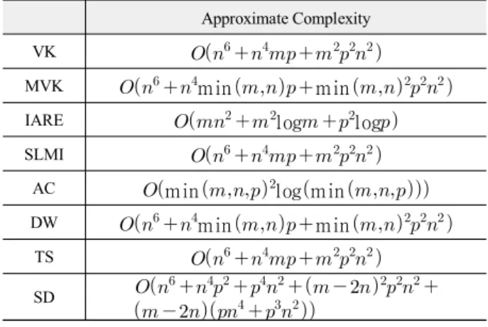
Since the computational complexity depends on the number of variables, the matrix size in LMI and the existence of iterations, they are summarized in table-1. The associated computational complexities are summarized in table-2. They are valid when associated parameters are asymptotically large since it is presented as big O complexity. The complexity with parameters of small value is likely to depend on scaling factors which are not shown in big O complexity representation. Thus, we will go back to this issue through measuring processing time for some system configurations in the next section. Nonetheless, the maximum order in big O can be representing how large the complexity it may be. From this perspective, AC algorithm is likely to have the smallest complexity while IARE algorithm does the second.
Table 1. The summary of the number of variables, the matrix size in LMI, and the existence of iterations for each method.
The number of variables
The matrix size in LMI
Existence of iterations
VK × Yes
MVK min × Yes
IARE N/A Yes
SLMI × Yes
AC N/A No
DW min
min × No
TS ×
× No
SD
i f ≥
× No
Table 2. The complexity of the methods for designing a static output feedback controller.
Approximate Complexity VK MVK min min IARE log log
SLMI AC min logmin
DW min min TS SD
Ⅴ. Numerical Experiments
In this section, we compare the performance of the considered control algorithms in terms of stabilizability. To this end, matrices, and are independently and identically generated from standard normal distribution. For each system configuration represented as a tuple the number of events that a controller provides stability is counted over 10000 system realizations. The stability of the derived closed loop system was judged from testing whether the maximum absolute of eigenvalue of the closed loop system is less than 1 or not. The maximum number of iterations for VK, MVK, and IARE were limited to 100 to reduce simulation time, since convergence seemed to be achieved with several iterations. in (8) for SLMI algorithm was set from -0.5 to 0.4 with 0.1 step.
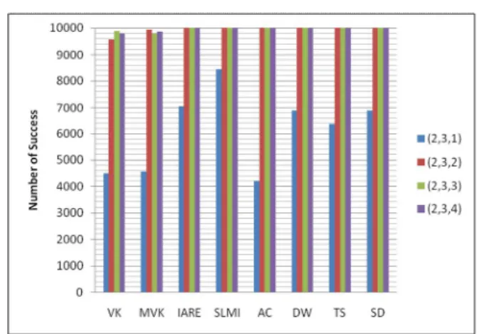
In figure-6, stabilizability of the considered algorithms is
assessed for increasing number of outputs while fixing and as 2 and 3 respectively. It is observed that the stability of the closed loop system controlled by all the considered algorithms was achieved in most cases when the number of outputs is greater than or equal to the number of states. There are several cases that VK and MVK algorithms does not provide stability even when
≥ , which be attributed to local convergence with iterations.
SLMI algorithm shows the best performance for (2,3,1), which can be attributed to trying several design methods with different scalars. The worst performance of AC can be attributed to a random controller for (2,3,1). It is noted that both DW and SD algorithm exploit the gain matrix structure of a state feedback controller, which may help to find a stabilizing output feedback controller.
The performance of the considered algorithms is compared in figure-7 for increasing number of inputs with fixing and as 2 and 4 respectively. It is observed that considerable number of failures in stabilizing a system happen with IARE, SLMI, and AC algorithms for (2,1,4). The performance degradation with AC for this system configuration can be attributed to the fact that it operates as a random controller while further research is needed to find out the cause for IARE and SLMI algorithms. It is also noted that VK has significant number of failures for (2,5,4). Even though VK and MVK has the same LMI constraint size, they have different dimension for optimizing variables. We conjecture that the reduction in the dimension of optimizing variables can have less numerical problems which make MVK work fine for (2,5,4).
Performances with increasing number of states are also shown in figure-8 for and . Drastic performance degradation is observed as increases. VK, MVK, and AC algorithms show relative worse performance while AC algorithm does the best performance for and
.
Fig. 6. Performance with increasing number of inputs.
Fig. 7. Performance with increasing number of outputs.
Fig. 8. Performance with increasing number of states.
Fig. 9. Comparison of the processing time of controller design for the number of states.
1 2 3 4 5 6
10-2 10-1 100 101 102 103 104
The number of states
Proecssing Time
VK MVK IARE SLMI AC DW TS SD
Fig. 10. Comparison of the processing time of controller design for the number of inputs.
Fig. 11. Comparison of the processing time of controller design for the number of outputs.
To assess the complexity, processing time for calculating a gain matrix was measured for each system configuration over 1000 random system realizations while simulation condition is same as one previously mentioned unless otherwise stated. A computer with Intel Core i5-4690 CPU, 8.0GB RAM, and 64bit Windows 7 is used. The measurement of processing time was executed sequentially while leaving alone the computer until it was finished.
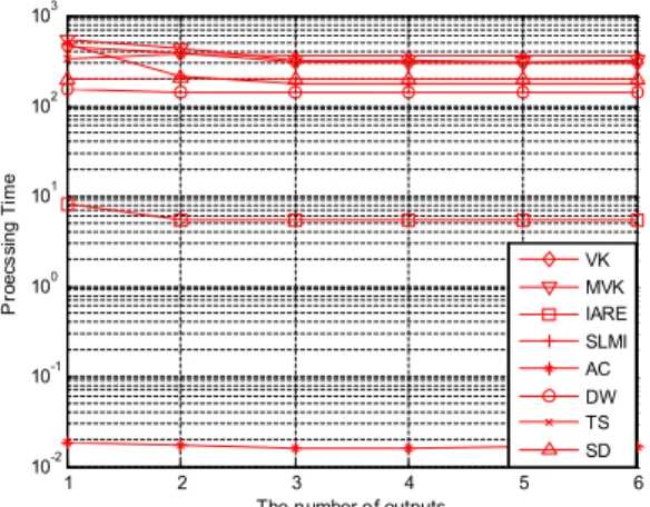
In figure-9, the processing time for designing a static output feedback controller was compared for increasing number of states while and . As expected from big O complexity analysis, AC algorithm shows the smallest processing time while the IARE algorithm takes the second.
Other algorithms seem to have similar order of complexity while DW, TS, and SD have relatively smaller complexity. It is
observed that VK, MVK, and SLMI algorithms have larger complexity with increasing number of states. As the number of states increases with the fixed and required number of iterations increases proportionally in addition to the increase in the complexity due to increased dimension in LMI.
It is also found that the complexity of the IARE algorithm is quite insensitive to the number of states. These results may be attributed to the parallel processing in a SW package.
In figure-10, the processing time for designing a static output feedback controller was compared for increasing number of inputs while and . SLMI algorithm is found to have relative increase in processing time when while the complexities of other algorithms do not vary much over the different number of inputs. Increase in the processing of SLMI algorithm is due to the increased number of iterations which runs independently with different scalar. It is observed that the complexities of other algorithms do not vary much over the different number of inputs. In figure-11, the processing time for designing a static output feedback controller was compared for increasing number of outputs while and . It is observed that every iterative algorithm has increased processing time due to increased number of iterations when . It is also noted that AC algorithm have relatively consistent complexity for every system configuration considered. This result is attributed to the fact that its complexity depends on min .
Ⅵ. Conclusions
In this paper, a class of existing states of arts in the design of a static output feedback controller was presented in a unified way so that it could be applicable to any system configuration. The efficiency of the designs was assessed in terms of stability and complexity associated with it. Among eight algorithms, AC algorithm has the smallest complexity for all considered system configurations. SLMI algorithm seems to achieve the best stability in most cases while its complexity is relative much larger than AC and IARE algorithm. It will be desirable to select an algorithm depending on a system configuration in consideration of complexity. For example, IARE algorithm and AC algorithm can be choices for the small number of outputs and the small number of inputs respectively.
There are several things to note from reviewing the methods for designing the static output feedback controller. First, IARE and AC algorithms are not associated with Lyapunov matrix.
This means that the complexity of Lyapunov-based method can
1 2 3 4 5 6
10-2 10-1 100 101 102 103
The number of inputs
Proecssing Time
VK MVK IARE SLMI AC DW TS SD
1 2 3 4 5 6
10-2 10-1 100 101 102 103
The number of outputs
Proecssing Time
VK MVK IARE SLMI AC DW TS SD
be limited by calculating Lyapunov matrix. However, it is a nontrivial problem to extend AC algorithm or direct optimization method on the eigen-value to a multi-objective control problem, which calls for further research [9]. A necessary and sufficient condition for the existing algorithms with various system configurations needs to be studied more theoretically. For example, considered algorithms have different characteristic for . The practical consideration of complexity is also needed. In many control problems, the number of states or the number of outputs are often not very large. Thus, complexity based on big O may not be enough to give an accurate estimate on complexity. In addition, parallel processing may have some impact on the complexity when the processing time is limited and the sufficient number of programmable logics is available. Thus, more generic model for the complexity on designing a controller needs to be paid attention.
The implication of the simulation results is limited except that what kind of algorithms may perform well in various system configurations. Since each algorithm has different structures and it is found from one satisfying LMI, it is not straightforward to explain why one algorithm works better while another algorithm works worse. However, performance comparison through simulations can be a starting point to study theoretically why one type of algorithm works better than the other algorithm. Even though we considered stability only, further numerical comparison is called for to reveal whether the algorithm providing the best stability performance can work best in control problems in terms of performance and ∞ performance.
Acknowledgement
이 논문은 2018년도 정부(미래창조과학부)의 재원으로 한국 연구재단의 지원을 받아 수행된 기초연구사업임(과제번호 :NRF-2017R1A2B4007398)
References
[1] N. Jazdi, “Cyber physical systems in the context of Industry 4.0,” in Proceeding of Automation, Quality and Testing, Robotics, Cluj-Napoca: Romania, May 2014.
[2] E. A. Lee, “Cyber Physical Systems: Design Challenges,” in Proceedomg of 11th IEEE International Symposium on Object Oriented Real-Time Distributed Computing (ISORC), Orlando: FL, May 2008.
[3] J. Sztipanovits, X. Koutsoukos, G. Karsai, N. Kottenstette, P.
Antsaklis, V. Gupta, B. Goodwine, J. Baras, and S. Wang,
“Toward a Science of Cyber-Physical System Integration,”
Proceedings of the IEEE, Vol. 100, No. 1, pp.29-44, Jan.
2012.
[4] M. Mizoguchi, and T. Ushio, “Output Feedback Controller Design with Symbolic Observers for Cyber-physical Systems,” in Proceeding of the The First Workshop on Verification and Validation of Cyber-Physical Systems, Reykjavik: Iceland, pp.37-51, June 2016.
[5] V. Blondel, M. Gevers, and, A. Lindquis, “Survey on the State of Systems and Control,” European Journal of Control, Vol. 1, No. 1, pp.5-23, 1995.
[6] V.L.Syrmos, C.T.Abdallah, P.Dorato, and K.Grigoriadis,
“Static output feedback-A survey“, Automatica, Vol. 33, No .2, pp.125-137, Feb. 1997.
[7] M. S. Sadabadia, and D. Peaucelleb, “From static output feedback to structured robust static output feedback: A survey,” Annual Reviews in Control, Vol. 42, pp.11-26, 2016.
[8] T. Iwasaki, R. E. Skelton, and J. C. Geromel, “Linear quadratic suboptimal control with static output feedback,”
Systems & Control Letters, Vol. 23, No. 6, pp. 421-430, Dec. 1994.
[9] J. V. Burke, D. Henrion, A. S. Lewis, and M. L. Overton,
“Stabilization via Nonsmooth, Nonconvex Optimization,”
IEEE Transaction on Automatic Control, Vol. 51, No. 11, pp. 1760-1769, Nov. 2006.
[10] J. Fiala, M. Kocvara, M. Stingl, “PENLAB: A MATLAB solver for nonlinear semidefinite optimization,” [Internet].
Available: https://arxiv.org/pdf/1311.5240.
[11] F. Palacios-Quinonero, J. Rubio-Massegu, J. M. Rossell, and, H. R. Karimi, “Recent advances in static output-feedback controller design with applications to vibration control of large structures,” Modeling Identification and Control, Vol. 35, No. 3, pp. 169-190, Mar. 2014.
[12] A. I. Zecevic, and D. D. Siljak, “Control design with arbitrary information structure constraints,” Automatica, Vol. 44, No. 10, pp. 2642-2647, Oct. 2008.
[13] L. El Ghaoui, and V. Balakrishnan, “Synthesis of fixed-structure controllers via numerical optimization,” in Proceeding of the 33rd IEEE Conference on Decision and Control, Lake Buena Vista: FL, pp. 2678-2683, Dec. 1994.
[14] T. Iwasaki, “The dual iteration for fixed-order control,”
IEEE Transaction on Automatic Control, Vol. 44, No. 4, pp.
783-788, Apr. 1999.
[15] I. Masubuchi, A. Ohara, and N. Suda, “LMI-based
![Fig. 3. Algebraic controller algorithm [20].](https://thumb-ap.123doks.com/thumbv2/123dokinfo/5188974.350753/5.892.464.812.123.251/fig-algebraic-controller-algorithm.webp)
![Fig. 4. Two-steps algorithm [22].](https://thumb-ap.123doks.com/thumbv2/123dokinfo/5188974.350753/6.892.459.807.104.209/fig-steps-algorithm.webp)