IEG 환경지질연구정보센터

Vol. 16, No. 4, p. 447 − 454, December 2012 DOI 10.1007/s12303-012-0039-y

ⓒ The Association of Korean Geoscience Societies and Springer 2012

Typhoon-generated microseisms observed from the short-period KSRS array

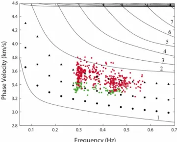
ABSTRACT: The seismic-noise data recorded on 19 vertical-com- ponent short-period seismometers of the KSRS seismic array are analyzed (1) to determine whether typhoons in the Pacific Ocean can be tracked accurately, and (2) to explore the seismic phases comprising the noise field recorded at the array. For our tests, two super typhoons, Sinlaku and Rammasun of 2008, were selected on the basis of their strength and wide azimuthal coverage from the seismic array. To track the source of DF microseisms, f-k analysis was applied to the KSRS data to estimate the back azimuth of the 0.2–0.7 Hz noise field (DF microseisms). These computed back azi- muths show good agreement with the known values to the centers of the NW Pacific typhoons. This clearly indicates that these typhoons were the main source of microseisms during their passing. The seismic phases in our DF microseism band are investigated with the phase velocities from our f-k analysis. The estimated horizontal phase velocities range from 3.2 to 3.8 km/s, with an average of about 3.5 km/s. This indicates that the major phases of the observed DF microseisms are surface waves consisting of mostly P-SV Mode 1 and Mode 2—in amplitude ratio A

/A

≈ 1/3—and possibly some Mode 3.

Key words: KSRS, directivity, typhoon, f-k analysis 1. INTRODUCTION

Seismometers record continuous and systematic vibra- tions due to ocean activities. These continuous vibrations are called microseisms and have two prominent peaks in the frequency ranges 0.05–0.1 Hz (primary or single-frequency microseisms, SF) and 0.1–0.5 Hz (secondary or double-fre- quency microseisms, DF).

It has long been recognized that intense cyclonic storms at sea produce strong winds that transfer atmospheric energy into oceanic gravity waves, and part of that energy couples with the solid earth to generate diffuse seismic waves, or microseisms, propagating in the acoustic system formed by the ocean and solid structure below. Investigation of microseisms

is now recognized as an important means of monitoring cli- mate-change effects, of locating storms (Bromirski, 2001), and of imaging the earth structure (Shapiro et al., 2005;

Kang and Shin, 2006).

The relation between oceanic storms (or moving pressure lows) and microseisms was studied by Gutenberg (1931), and the cyclones near North America were first successfully tracked with observed microseism data (Gilmore, 1946) using the tripartite method (Ramirez, 1940). However, research on the source of microseisms was only moderately success- ful until array seismology (summarized by Rost and Thomas, 2002) became practical in the 1960s. Since then, array- based studies of noise have been more successfully focused on both the sources of microseisms and the composition of seismic phases within these arrivals.

Sources of primary microseisms near the coastlines of the North Atlantic and Pacific Oceans were detected using a wide-angle triangulation approach (Cessaro and Chan, 1989).

Location of source areas of secondary microseisms, that are observed at continental stations, has caused debates con- cerning whether these microseisms are generated mainly along the coast (Bromirski, 2001; Bromirski and Duenne- bier, 2002; Bromirski et al., 2005), or whether they are also generated in deep-sea regions (Cessaro, 1994; Stehly et al., 2006; Kedar et al., 2008).

Recent array techniques using the body waves from a continuous-noise source, also allow location of the sources (Gerstoft et al., 2006; Zhang et al., 2010) and show that there exist seasonal variations of the source area (Gerstoft and Tanimoto, 2007; Koper et al., 2009). However, studies that track moving pressure lows, based on array techniques, are not common.

Backus et al. (1964) analyzed the noise data and found higher-mode Rayleigh waves with phase velocities of 3.5–

4.5 km/s within the period range 0.2–1.0 s. They also reported the presence of teleseismic P waves in the seismic noise Woo-Dong Lee

Bong-Gon Jo*

Fred Schwab Sat-Byul Jung

Department of Earth and Environmental Science, School of Science and Technology, Chonbuk National University, Jeonju 561-756, Republic of Korea

Department of Earth and Environmental Science, School of Science and Technology, Chonbuk National University, Jeonju 561-756, Republic of Korea

Institute of Earth and Environmental System, Chonbuk National University, Jeon ju 561-756, Republic of Korea Department of Earth and Space Sciences, University of California Los Angeles, Los Angeles, California 90095-1567, USA

Department of Earth and Environmental Science, School of Science and Technology, Chonbuk National University, Jeonju 561-756, Republic of Korea

*Corresponding author: [email protected]

(Backus, 1966). Lacos et al. (1969) demonstrated that the microseism wavefield consists of fundamental-mode Ray- leigh and Love waves at periods longer than 7 s. Recent studies have shown that at shorter periods, there is a com- plicated mixture of fundamental-mode surface waves, higher-mode surface waves, and body waves (Bonnefoy- Claudet et al., 2006; Koper et al., 2010; Gerstoft et al., 2008; Koper and de Foy, 2008; Landes et al., 2010; Zhang et al., 2010).

Strong DF microseism peaks during Korean summer sea- son were correlated with the presence of Pacific typhoons (Sheen et al., 2009). In this study, we carry out a survey of the noise field using the KSRS seismic array. The seismic array technique is a powerful tool for the study of noise sources; it provides accurate information on both the direc- tion of propagation and wave velocity of the incoming seis- mic noise as it crosses the array. Our research target is two- fold: (1) to determine whether typhoons in the Pacific Ocean (east and south of Japan) can be tracked accurately using the short-period KSRS array, and thereby verifying that typhoons are sources of recorded microseisms, and (2) to examine the seismic composition of the noise field recorded

at the KSRS array. Our report is the initial analysis of using the KSRS array to track typhoons.

2. DATA AND METHOD

In the year 2008 there were 32 tropical cyclones (or mov- ing pressure lows) in the NW Pacific, 11 of which reached

“Typhoon” level. We have studied the second (“Ramma- sun”) and eighth (“Sinlaku”) of these typhoons (Fig. 1).

This pair was selected on the basis of (1) their strength, both being Category 4-equivalent, “Super Typhoons”, and of (2) their wide azimuthal coverage at, and ease of distinguishing them with, the KSRS array. (We use the 2009 tropical-cyclone classification of the Hong Kong Observatory, which is given in Table 1) This array consists of 19 vertical-component, short-period instruments located at Wonju, South Korea.

The seismometers are within a circle of diameter—maxi- mum array aperture—10.1 km, and the minimum inter-sta- tion separation is about 2 km (Fig. 1). The 19 short-period instruments with resonance frequency at 1 Hz are identical, and measure velocity; and to the accuracy required in the current study, the phase response of all the instruments is

Fig. 1. Index map. This shows the Korean seismic array KSRS, and the typhoon-center tracks of Sinlaku and Rammasun of 2008. The circles repre- sent effective diameters of strong wind of each typhoon. (The effective diam- eter of strong wind is the area inside the typhoon, having a speed greater than 54 km/h.) The typhoon locations with circle and square symbols corre- spond to the same symbols in Figure 3.

The inset shows the array configura-

tion of the 19 vertical, short-period

instruments of the KSRS array.

assumed to be the same.

To prepare for analysis, these velocity records are filtered using a three-pole Butterworth band-pass filter with corners at 0.2 and 0.7 Hz, and each window is individually detrended and tapered with a Hanning window. Even though the fre- quency range used in this study is lower than the resonance frequency of the KSRS instruments, the DF microseism energy in the frequency range of 0.2–0.7 Hz appears dom- inant in the recorded seismogram during the days of min- imum seismic intensity shown in Figure 3. To the array’s spatial distribution of recorded and processed seismograms, frequency-wavenumber ( f-k) analysis is applied to compute f-k spectra for two different sizes of time windows, 6.5 s and 720 s.

The complete details of this procedure will be found in Rost and Thomas (2002) and references therein. This pro- vides us with the direction and horizontal velocity of mono- chromatic waves passing across array KSRS, i.e., the vector (horizontal) wavenumber at the array for the frequency band and time window of the processed set of recordings.

For this purpose, a modified version of the Generic Array Processing (GAP) Software Package (Koper, 2005) is used to analyze the KSRS array data. The frequency band ana- lyzed for the array was carefully chosen to avoid spatial aliasing. For the KSRS short-period network, the inter-sta-

tion distance ( ∆x ≈ 2 km) is quite constant. Thus the Nyquist wavenumber (1/2 ∆x) is 0.25 km

. With the slowness grid ranging between –45 to +45 s/ ° in S

and S

domain, and a center frequency of 0.5 Hz at which to calculate f-k spectra, a maximum wavenumber within the search bounds is about 0.2 km

. The maximum wavenumber for the center fre- quency is lower than the Nyquist wavenumber of the array so that the spatial aliasing for 0.5 Hz is not a problem for Table 1. Classification of tropical cyclones

Tropical Cyclone classification

Maximum 10-minute mean wind near the center Tropical Depression up to 62 km/h

Tropical Storm 63 to 87 km/h

Severe Tropical Storm 88 to 117 km/h

Typhoon 118 to 149 km/h

Severe Typhoon

150 to 184 km/h Super Typhoon

185 km/h or above

a

New categories starting 2009

Fig. 2. Array response functions (ARF) of KSRS. ARFs to a vertically incident wave at frequencies of 0.2 Hz, 0.5 Hz and 0.7 Hz are plotted. S

and S

indicate the slownesses in east-west and north-south directions, respectively.

Fig. 3. Spectrograms. This shows the temporal and spectral vari- ations of normalized power spectra in dB during the two 2008 typhoons, Sinlaku (a) and Rammasun (b). The two dashed hori- zontal lines at 0.2 and 0.7 Hz indicate the frequency range of DF microseisms. FFT is applied to 1000-second time windows with 50%

overlapping, and the normalized power spectral density (PSD)

have been smoothed in the temporal and spectral domains. The

spectrogram is a time-varying spectral representation that shows

how the spectral density of a signal varies with time.

the array. This point is illustrated in Figure 2. The theoret- ical array responses of KSRS, for vertically incident plane waves of frequency 0.2, 0.5, and 0.7 Hz are shown in Fig- ure 2. The ideal response would be a delta function at the origin, but due to the spatially discrete array with the finite number of stations, the response becomes broad and side lobes appear (Koper et al., 2010).

The application of f-k analysis is limited to short-time window, and in our case the window sizes are 6.5 s and 720 s.

To find optimal slowness vectors along the extended seis- mogram, the sliding-window technique (Rost and Weber, 2001) is applied. In this technique, a constant short-time window is shifted along the extended seismogram with a constant step size. In our case, the time-window was shifted along the seismograms by overlapping 50 percent of the time window size. The optimal slowness vector gives the highest beam-forming power for waves incident to the array, and for that the grid is set up in a Cartesian coordinate system, which is defined by ±45 s/ ° with the increments of 0.5 s/ ^° .

At array KSRS, the results of the f-k procedure are, for a given frequency and time window, the magnitude and direc- tion of the ray parameter (or horizontal phase slowness S).

These are given in terms of the east-west component S

, and north-south component S

: S = in seconds per degree, back azimuth = tan

( S

/ S

) in clockwise radians from north, with the apparent horizontal phase velocity, in kilometers per second, given by c = K/S. To the accuracy required here, we can define K as 40,000 km/360 ^° . 3. RESULTS

3.1. Tracking the Source of Microseisms

Locating the source of cyclone-generated microseisms can be attempted by using the intersection method with back azimuths computed from more than one array (Ces- saro, 1994). In the current study, however, we already know the time-dependent location of the typhoon’s center, and hence the time dependent direction from KSRS to that cen- ter. Our first research target is then to use microseisms recorded at KSRS to compute this time-dependent direc- tion, and hence by comparison with the known directions, to determine whether the center of typhoons in the Pacific Ocean (east and south of Japan) can be tracked accurately using this short-period array in the center of the Korean peninsula.

Whatever the exact mechanism of typhoon excitation of microseisms, we begin this study with the assumption that the spatially-distributed source has an effective centroid of excitation on the line between KSRS and the typhoon’s cen- ter. In our computations, first we check the frequency range where microseismic energy exists, and spectral and tempo- ral variations of the noise are investigated. We find that

whenever one of our two typhoons exist, DF microseisms are clearly observed in the spectrograms shown in Figure 3 of a short-period KSRS seismometer, and that most of the energy is concentrated within the frequency band 0.2–0.7 Hz.

These spectrograms show a clear continuation of microseism energy over time.

In this investigation, Sinlaku and Rammasun were stud- ied from September 9 to September 20, 2008, and from May 11 to May 13, 2008, respectively, after the moving areas of low pressure developed fully from Tropical Storm to Typhoon. The tropical cyclone, Sinlaku, was declared first a Tropical Depression located east of the Philippines on September 8

, developed to Typhoon status, and made landfall September 13

on Taiwan with winds of 170 km/h which made it a Category 2-equivalent typhoon. As Sinlaku moved through Taiwan, it turned to the northeast on Sep- tember 15

, moved eastward to the South China Sea, and started toward Japan (Fig. 1). It weakened after the 13

, but attained Typhoon status again on September 16

, and by the 21

was classified as a pressure low. Rammasun started as an area of low pressure on May 7, 2008, slowly moved northward and quickly developed to Typhoon level on May 9

, and continuing on a northerly path it finally attained Super Typhoon status on May 10

with a peak wind speed of 194 km/h and minimum pressure of 915 hPa. Then it began weakening, changed its direction toward the east just below the Japanese island arc (Fig. 1), and by May 13

was downgraded to a pressure low.

To assess the correlation between the seismic noise field recorded at KSRS, and a given typhoon’s movement, we compared the computed back azimuth from the noise, with the known direction to the typhoon’s center. For each typhoon, we began with a preliminary examination of the f- k spectra to see if they looked reasonable enough to deter- mine slowness vectors from the KSRS data, without any spatial aliasing. We then selected four specific time win- dows for which the f-k spectra were computed in the fre- quency range 0.2–0.7 Hz, and the resulting back azimuths are compared with the known values to the typhoon center in Figures 4a and c for Sinlaku, and in Figures 4b and d for Rammasun.

In actual application, the sliding-window technique (Rost

and Thomas, 2002) is used to search for the optimum com-

bination of phase slowness and back azimuth from the f-k

spectra. Two different time-window widths, 6.5 s and 720 s,

are employed in the search for directional constraints. We

selected peaks of f-k spectra for each time window, and

these are the plotted results in Figures 4a and b. The grey

dots and red dots represent the computed back azimuths

from window widths 6.5 s and 720 s, respectively. The

dashed blue lines are fitted curves for the computed back

azimuths of the 6.5 s windows, and the solid blue lines are

the known back azimuths to the center of the typhoons. The

computed back azimuths from the time window 6.5 s wide

S

+ S

have a variance of 50 ^° , which becomes smaller as the width of the time window is increased to 720 s (Figs. 4a and b).

The result for 720 s is a variance of about 20 ^° and tracks the center of the typhoons better. There are, however, consid- erable misfits between the known directions to the typhoon locations, and the computed directions between locations

“c” and “d” of Sinlaku in Figure 4a. The obvious reason for this misfit is that the typhoon fell on Taiwan and mainland China, with only the eastern side of Sinlaku becoming the effective source of the recorded microseisms. That is, the spatially distributed source of microseisms—the atmosphere- ocean interaction of the typhoon—temporarily became a centroid that was no longer on the line connecting KSRS and the typhoon’s center (see Fig. 1).

These back azimuth results clearly demonstrate that Sin- laku and Rammasun governed the microseism noise fields on the Korean peninsula during the lives of these typhoons.

3.2. Seismic Phase Composition of Noise Field

To represent the back azimuth and slowness ranges together, Figure 5 collects the results of the f-k analysis applied to the 720 s time window in polar plots. These computed hori- zontal phase slownesses for microseisms range from 29 s/ ° to 34–35 s/ ^° . This corresponds to the horizontal phase-velocity range of 3.2–3.8 km/s, with an average of about 3.5 km/s.

Thus the largest source of noise at KSRS arrives with the apparent velocity of surface waves. For interpretation, these results are redisplayed in Figure 6 as the more common phase-velocity dispersion, with Modes 1 −7 of P-SV (Ray- leigh-type) surface waves included for reference. (For our approximation to the structure beneath array KSRS, we use the upper 12 km from Jung et al. (2011) and a standard shield (Harkrider, 1970) below 12 km; from 12–40 km this appears to be close enough to the CHJ model of Chang and Baag (2005).

Rather than attempt to assign velocity and frequency error bars to each of the individual plotted points in Figure 6, we use the scatter of the complete set of points to assess Fig. 4. Comparison of computed back azimuths to the centers of the two typhoons and corresponding f-k spectra. Panels (a) and (b):

Back azimuths computed from f-k analysis are compared with the direction to typhoon eyes from the KSRS station. The solid blue line represents back azimuth to the typhoon centers. The dashed blue line indicates estimated back azimuths using seismic noise data. Panels (c) and (d): The panels show f-k spectra computed from 720 second time windows. Highest beam power in the f-k spectra is presented in black color. The back azimuths are measured clockwise from north to maximum beam power. The red line indicates the real direction to a typhoon center for a given time window. The alphabetic symbols in the lower panel correspond to those in the upper panel.

Fig. 5. Slowness vectors. For microseism phases crossing array

KSRS, Panels (a) and (b) show the slowness vectors for Sinlaku

and Rammasun, respectively.

a hypothetical single apparent phase-velocity dispersion, with the variation from that curve being our estimate of its accuracy. The point scatter clearly shows the frequency dependence we expect, so we focus only on the phase-veloc- ity distribution which has a range of about ±0.2 km/s at each frequency. In a manner similar to what was originally done for Mode 1-Mode 2 interference of long-period SH (Love-type) surface waves (Thatcher and Brune, 1969;

Boore, 1969), we estimate the fractional amounts of Mode 1 and higher modes (that cross KSRS as microseisms), by summing Mode 1 and Mode 2 at a given value of time t (well away from an interference minimum). For amplitude A, angular frequency ω, and phase velocity c, we represent the vertical component of ground-motion displacement as

(1)

and over a ξ range of 20 km determine the apparent wave- length between peaks of f(ξ), which yields

apparent phase velocity = apparent wavelength (2) for any selected ratio of A

and A

. With equal amplitudes A

/ A

= 1/1 we obtain the black squares in Figure 6, and A

/ A

≈ 1/3 with the black triangles. Obviously, there is about three times the Mode 1 amplitude in the higher modes, in the frequency range 0.30–0.55 Hz.

The comments above treat all of the measured phase velocities—those from both Sinlaku and Rammasun—together.

However, reference to Figure 6 will show that the measure- ments from Sinlaku (red dots) and those from Rammasun (green dots) clearly separate into two distinct groups: the Sinlaku measurements yielding an amplitude ratio A

/ A

≈ 1/3, and those from Rammasun, A

/ A

≈ 1/1.

Although this is the first evidence of such a separation, it is rather convincing, and extremely interesting in its impli- cation that the two typhoons are exciting different modal signatures. Actually we should expect something of this sort, with Sinlaku mainly centered over the shallow waters of the continental shelf, and Rammasun centered over the deeper ocean seaward of the continental slope, assuming that the cyclonic excitation of microseisms takes place rel- atively near its center.

4. CONCLUSIONS AND DISCUSSION

We have investigated the noise field recorded at the short- period KSRS array, and using f-k analysis have estimated the directivity of the incident field crossing KSRS in the frequency range 0.2–0.7 Hz. We found that the computed back azimuths of these DF microseisms follow rather well the known back azimuths to the moving centers of NW Pacific, 2008 typhoons Sinlaku and Rammasun. This clearly indicates that typhoons are an effective cause of DF microseisms. The computed back azimuths agreeing rather well with the known back azimuths to each moving typhoon’s center, however, only tell us that the effective centroid of the microseism’s excitation is approximately on the oceanic portion of the line connecting KSRS and Sinlaku’s center, or KSRS and Rammasun’s center. This is sufficient, how- ever, for KSRS back azimuth tracking of NW Pacific typhoons (at least in the azimuth range of 110° to 220° clockwise from north). It gives us an important means of monitoring the weather in the NW Pacific Ocean in real time, and of reconstructing past storm activities for those times during which we do not have oceanic, weather data.

Our successful KSRS tracking of NW Pacific typhoons (west and south of Japan) can be compared with the initial tracking (Gilmore and Hubert, 1948, Tab. 5, 6, 8, 9, 10, 11) in the area containing our paths; a tracking that they carried out with a highly specialized tripartite array located on Guam. Our average difference between the calculated back azimuths at KSRS and the known values to the centers of Sinlaku and Rammasun is about 11°; from the tabulated dif- ferences in the 1948 report, the average difference is about 4 ± 2°. These differences have been scaled to a common, array-to-typhoon center distance of 1000 km; and, we have neglected the differences measured for the second typhoon in Tab. 9 of the 1948 report, as being far outside of the com- mon range from the other six 1947 typhoons. To assess the variation between the 1948 and 2008 differences, we note f ξ ( ) A =

cos ( ωt k –

( )ξ ω ) A +

cos ( ωt k –

( )ξ ω )

A

cos ωt ω c

( ) ω ---

⎝ ⎠

⎛ ⎞ξ

⎝ – ⎠

⎛ ⎞ A

cos ωt ω

c

( ) ω ---

⎝ ⎠

⎛ ⎞ξ

⎝ – ⎠

⎛ ⎞

+

=

ω 2 π ---

Fig. 6. Theoretical and observed phase velocity at KSRS. The

solid curves and numbers on the curves indicate P-SV theoretical

dispersion curves for the continental structure. Red and green

closed circles are observed phase velocities of Sinlaku and Ram-

masun, respectively. Triangles, squares, and circles between the

Mode 1 and Mode 2 dispersion curves are computed dispersion

curves with the amplitude ratios A

/A

≈ 1/3, 1/1, 4/1, respectively.

that Gilmore’s 1953a report explains that the initial back azimuth measurements of the 1940s naturally focused on the cyclones yielding the best results, and that cyclones in other azimuth ranges from his tripartite arrays gave much poorer results—without correcting for lateral refraction of the microseisms (Gilmore, 1953b). With only Sinlaku and Rammasun in our initial tests at KSRS, and the associated complex structure for the microseisms to traverse, lack of correction for lateral refraction has surely affected our com- puted differences. Added to that, the instruments used by Gilmore (1954) were highly specialized for microseismic research; an advantage not possessed by the instrumentation at KSRS. These explanations do, however, indicate obvious directions for improvement in our microseism recording technique, and in the processing of our data. These avenues of improvement, plus the associated questions stated and implied by Cessaro (1994) and Friedrich et al. (1998), have led us to expand the current study of typhoon-generated microseisms recorded at the KSRS array.

It is interesting to note that for the 1000 km separation of array and typhoon center, the characteristic, eyewall radii of 30–65 km give a maximum-difference range of 1.7–3.7°

and an average-difference range of 1.1–2.4°, if that average is for a time-random angular location within the typhoon's eyewall—within the typhoon's region of maximum wind, and hence within the areal band of maximum oceanic gravity waves generated by the typhoon. Thus the 1948 average- difference range of 4 ± 2° gives us the beginning of quan- titative support for locating a logical typhoon area from which DF microseisms can be generated by the standing- wave mechanism of Miche (1944), Longuet-Higgins and Ursell (1948), and Longuet-Higgins (1950). One purpose of the above improvements in our KSRS microseism investi- gations, is to restrict further the bounds on this location.

The recorded microseisms crossing the array KSRS, caused by 2008 typhoons Sinlaku and Rammasun, had vertical- component horizontal phase velocities in the frequency range 0.30–0.55 Hz: (1) that had the correct frequency dependence for a combination of P-SV Mode 1, Mode 2, and a small amount of Mode 3; (2) that could be fit with a theoretically-computed phase-velocity dispersion for Modes 1 and 2 in amplitude ratio of about A

/ A

≈ 1/3; and (3) that had an uncertainty of about 0.2 km/s. This is consistent with the literature survey given by Koper et al. (2010, pages 607–608), where the frequencies below our range tended to be represented mainly by Mode 1, and the frequencies increasing above our range, tended toward an average phase velocity of about 4.0 km/s, i.e., a combination of mainly higher modes. This suggests that the oceanic microseisms incident upon the coastal region, scatter into continental modes that sample the crust more or less uniformly over depth: at low frequencies this is accomplished by Mode 1 alone; as frequency increases and crustal-wave (Panza et al., 1972, Fig. 4) fundamental-mode energy migrates upward,

the first higher mode fills in the depth gap between the fun- damental mode and the bottom of the crust; and as fre- quency continues to increase, this process continues with successively higher mode numbers (see Knopoff et al., 1973, Fig. 9 for how this “fill-in” process would work for SH modes).

ACKNOWLEDGMENTS: We thank the Korea Earthquake Research Center (KERC) of Korea Institute of Geoscience and Mineral Resources for making the KSRS array data available. This work was supported by National Research Foundation of Korea (NRF) grant funded by Korean government (MEST) (No. 2012-0005092) and also the Korean Meteorological Administration Research and Development Program under Grant CATER 2012-8090. We thank two anonymous reviewers for comments that led to significant improvements in this report.

REFERENCES

Backus, M.M., 1966, Teleseismic signal extraction. In: Proceeding of the Royal Society Series A, 290, 343–367.

Backus, M., Burg, J., Baldwin, D., and Bryan, E., 1964, Wide-band extraction of mantle P waves from ambient noise. Geophysics, 39, 672–692.

Bonnefoy-Claudet, S., Cotton, F., and Bard, P.-Y., 2006, The nature of noise wavefield and its applications for site effects studies: A literature review. Earth-Science Reviews, 79, 205–227.

Boore, D.M., 1969, Effect of higher mode contamination on mea- sured Love wave phase velocities. Journal of Geophysical Research, 74, 6612–6616.

Bromirski, P.D., 2001, Vibrations from the “Perfect Storm”. Geochemistry Geophysics Geosystems, 2, doi: 10.1029/2000GC000119.

Bromirski, P.D. and Duennebier, F.K., 2002, The near-coastal microseism spectrum: Spatial and temporal wave climate relationships. Jour- nal of Geophysical Research, 107, 2166, doi: 10.1029/2001JB000265.

Bromirski, P.D., Duennebier, F.K., and Stephen, R.A., 2005, Mid- ocean microseisms. Geochemistry Geophysics Geosystems, 6, Q04009, doi:10.1029/2004GC000119.

Cessaro, R.K. and Chan, W.W., 1989, Wide-angle-triangulation array study of simultaneous primary microseism sources. Journal of Geophysical Research, 94, No. B11:15555-15563.

Cessaro, R.K., 1994, Sources of primary and secondary microseisms., Bulletin of Seismological Society of America, 84, 142–148.

Chang, S.-J. and Baag, C.-E., 2005, Crustal structure in southern Korea from joint analysis of teleseismic receiver functions and surface-wave dispersion. Bulletin of Seismological Society of America, 95, 1516–1534, doi: 10.1785/0120040080.

Friedrich, A., Krüger, F., and Klinge, K., 1998, Ocean-generated microseismic noise located with the Gräfenberg array. Journal of Seismology , 2, 47–64.

Gerstoft, P., Fehler, M.C., and Sabra, K.G., 2006, When Katrina hit California. Geophysical Research Letters, 33, L17308.

Gerstoft, P. and Tanimoto, T., 2007, A year of microseisms in south- ern California. Geophysical Research Letters, 34, L20304, doi:

10.1029/2007GL031091.

Gerstoft, P., Shearer, P.M., Harmon, N., and Zhang, J., 2008, Global P, PP, and PKP wave microseisms observed from distant storms.

Geophysical Research Letters, 35, L23306, doi: 10.1029/

2008GL036111.

Gilmore, M.H., 1946, Microseisms and ocean storms. Bulletin of Seismological Society of America, 36, 89–120.

Gilmore, M.H. and Hubert, W.E., 1948, Microseisms and Pacific

typhoons. Bulletin of Seismological Society of America, 38, 195–228.

Gilmore, M.H., 1953a, Amplitude distribution of storm microseisms.

In: Wilson, J.T. and Press, F. (eds.), Symposium on Microseisms.

National Academy of Sciences, National Research Council Pub- lication, 306, 20–32.

Gilmore, M.H., 1953b, Discussion. In: Wilson, J.T. and Press, F.

(eds.), Symposium on Microseisms. National Academy of Sci- ences, National Research Council Publication, 306, 16–18.

Gilmore, M.H., 1955, Operating Manual for Microseismic Research.

W.F. Sprengnether Instrument Company, Inc., Saint Louis, 41 p.

Gutenberg, B., 1931, Microseisms in North America. Bulletin of Seismological Society of America, 21, 1–24.

Harkrider, D.G., 1970, Surface waves in multilayered elastic media, Part II. Higher mode spectra and spectral ratios from point sources in plane layered earth models. Bulletin of Seismological Society of America, 60, 1937–1987.

Jung, H., Jang, Y. S., and Jo, B.G., 2011, Upper-Crust Shear-Wave Veloc- ity of South Korea Constrained by Explosion and Earthquake Data. Bulletin of Seismological Society of America, 101, 2819–

2832, doi:10.1785/0120110026.

Kang, T.S. and Shin, J.S., 2006, Surface-wave tomography from ambient seismic noise of accelerograph networks in southern Korea. Geophysical Research Letters, 33, L17303, doi: 10.1029/

2006GL027044.

Kedar, S., Longuet-Higgins, M., Webb, F., Graham, N., Clayton, R., and Jones, C., 2008, The origin of deep ocean microseisms in the North Atlantic Ocean. In: Proceedings of the Royal Society, Series A, 464, 777–793.

Knopoff, L., Schwab, F., and Kausel, E., 1973, Interpretation of Lg.

Geophysical Journal of the Royal Astronomical Society, 33, 389–404.

Koper, K.D., 2005, The Generic Array Processing (GAP) software package. Seismological Research Letters, 76, 226.

Koper, K., and de Foy, B., 2008, Seasonal anisotropy of short-period seismic noise recorded in south Asia. Bulletin of Seismological Society of America, 98, 3033–3045.

Koper, K.D., de Foy, B., and Benz, H., 2009, Composition and vari- ation of noise recorded at the Yellowknife Seismic Array, 1991-2007.

Journal of Geophysical Research, 114, B10310, doi: 10.1029/

2009JB006307.

Koper K.D., Seats, K., and Benz, H., 2010, On the composition of Earth’s short-period seismic noise field. Bulletin of Seismologi-

cal Society of America, 100, 606–617.

Lacoss, R.T., Kelly, E.J., and Toksöz, M.N., 1969, Estimation of seis- mic noise using arrays. Geophysics, 34, 21–38.

Landes, M., Hubans, F., Shapiro, N.M., Paul, A., and Campillo, M., 2010, Origin of deep ocean microseisms by using teleseismic body waves. Journal of Geophysical Research, 115, B05302, doi:

10.1029/2009JB006918.

Longuet-Higgins, M.S., and Ursell, F., 1948, Sea waves and microseisms.

Nature, 162 , 700.

Longuet-Higgins, M.S., 1950, A theory of the origin of microseisms.

Philosophical Transaction of the Royal Society London, Series A, 243, 1–35.

Miche, M., 1944, Mouvements ondulatoires de la mer en profondeur constante ou decroissante Annponts et chaussee. 114, 25–87, 131–164, 270–292, 396–406.

Panza, G.F., Schwab, F., and Knopoff, L., 1972, Channel and crustal Rayleigh waves. Geophysical Journal of the Royal Astronomical Society, 30, 273–280.

Ramirez, J.E., 1940, An experimental investigation of the nature and origin of microseisms at St. Louis, Missouri: Part two. Bulletin of Seismological Society of America, 30, 139–178.

Rost, S. and Thomas, C., 2002, Array seismology: methods and appli- cations. Review of Geophysics, 40, doi: 10.1029/2000RG000100.

Rost, S. and Weber, M., 2001, A reflector at 200 km depth beneath the NW Pacific. Geophysical Journal International, 147, 12–28.

Shapiro, N.M., Campillo, M., Stehly, L., and Ritzwoller, M.H., 2005, High resolution surface wave tomography from ambient seismic noise. Science, 307, 1615–1618.

Sheen, D.H, Shin, J.S., and Kang, T.S., 2009, Seismic noise level variation in South Korea. Geosciences Journal, 13, 183–190, doi10.1007/s12303-009-0018-0.

Stehly, L., Campillo, M., and Shapiro, N.M., 2006, A study of the seismic noise from its long-range correlation properties. Journal of Geophysical Research, 111, B10306, doi: 10.1029/2005JB004237.

Thatcher, W. and Brune, J.N., 1969, Higher mode interference and observed anomalous apparent Love wave phase velocities. Jour- nal of Geophysical Research, 74, 6603–6611.

Zhang, J., Gerstoft, P., and Bromirski, P.D., 2010, Pelagic and coastal sources of p-wave microseisms: Generation under tropical cyclones.

Geophysical Research Letters, 37, L15301, doi:10.1029/2010GL044288.

Manuscript received March 31, 2012

Manuscript accepted September 27, 2012