2003, Vol. 14, No.1 pp 119∼129
Logistic Model for Normality by Neural Networks
Jea-Young Lee1) ․ Seong-Won Rhee2)
Abstract
We propose a new logistic regression model of normality curves for normal(diseased) and abnormal(nondiseased) classifications by neural networks in data mining. The fitted logistic regression lines are estimated, interpreted and plotted by the neural network technique. A few goodness-of-fit test statistics for normality are discussed and the performances by the fitted logistic regression lines are conducted.
Keywords : Logistic regression, Neural networks, Activation function
1. Introduction
A logistic regression analysis may belong to one of many techniques for classification that divide data by the normal group(diseased) and abnormal group(nondiseased). Specially, in neural networks it is easy to accept but difficult to use results from a classification because the analysis process is greatly complicated and hidden. Using the special quality of the activation function concerned deeply in output result of the neural network analysis, we apply the results of neural networks for a classification to the logistic regression modelling.
On the other hand there are graphical methods for doing normality test such as Q-Q (quantile-quantile) plot and P-P (probability-probability) plot. Wilk and Granadesikan(1968) introduced probability plotting methods for the analysis of data and normality test. LaBrecque (1977) studied about a normality test based on nonlinearity on probability plot. Mage(1982) introduced some graphical methods for normality test. Lee, Woo and Rhee (1998) proposed a new graphical method named
1) Associate Professor, Department of Statistics, Yeungnam University, Gyongsan, 712-749, Korea
E-mail : [email protected]
2) Adjunt Assistant Professor, Department of Statistics, Yeungnam University, Kyongsan, 712-749, Korea
E-mail : [email protected]
a transformed quantile-quantile plot to test for normality. However it is less formal and the use of it alone could lead to spurious conclusion. To solve this kind of problem, Lee and Rhee(1999) proposed the goodness-of-fit test for normality through ROC analysis. They obtained the estimated sample variances, S2QQ and S2PP from residuals of the transformed Q-Q and the transformed P-P plots respectively. Also the comparisons with Shapiro and Wilk's(1965) W statistic, were conducted by Monte Carlo simulations. This paper is organized as follows.
Section 2 describes a method of neural networks for a classification in data mining and suggests a new logistic model of normal(diseased) and abnormal(nondiseased) classifications by neural networks. Section 3 considers a simulation studies and the performance by fitted logistic regression model. The final section is devoted to summary and recommendations.
2. Logistic Regression Model by Neural Networks
We consider only the classification problem about two classes such as the normal group CN and the abnormal group CA. Let the training data set be defined by
T ={( x ( n ) ,d ( n ) ) | n = 1, 2, … , N } (2.1) where x ( n) is a m-dimensional input vector for item n and N is the total number of cases or items used in this analysis. And d ( n) is a desired response or target output for item n such as
d(n)={1, 0. x ( n)∈ Cx ( n) ∈ CNA (2.2) In neural networks, the output of each node is made by the activation function.
Specially, the model of each neuron in multilayer perceptron has a nonlinear and smooth activation function. A commonly used form of nonlinearity is a sigmoidal nonlinear function(Haykin,1999) which is defined by the logistic function such as
ϕ ( v ) = 1
1 +e- a v . (2.3) where a is the slope parameter of the sigmoid function.
In figure 1, by varying the parameter a, sigmoid functions of different slopes
are illustrated. The results of the activation function from the output layer with a single node of a multilayer perceptron with the error back-propagation algorithm is often called by scores and denoted by ο( n),(∈[0 1]) n = 1, 2, … , N . These scores are characterized by
Figure 1. Sigmoid activation function (Haykin,1999)
d( n) =
{
1, ο( n) ≥ c 0. ο( n) < c(2.4)
where d( n) is the result of classification for item n and c is a constant. In the multilayer perceptron with the activation function which is equation (2.3), the range of ο( n) is [0, 1] and the constant c = 0.5. Then the classification rules are defined by:
① If a score ο( n) is great than or equal to 0.5, then the item n is classed to the abnormal class CA.
② If a score ο( n) is less than 0.5, then the item n is classed to the normal class CN.
The scores have been used to classify by the classification rules(① and ②) only. But we want to use these scores for a logistic modelling. Because these scores came from the activation function described in (2.3) of the multilayer perceptron. In statistical viewpoint, a final output d( n) is the estimation of the desired responsed( n). That is, the event such as d( n) = 1 is equivalent to
ο( n) ≥ c. So, the probability form is formulated by
Pr [ d( n) = 1] = Pr [ ο( n) ≥ c], (2.5) and
Pr [ d( n) = 0] = Pr [ ο( n) < c]. (2.6) Then we define a new logistic regression model by neural networks, from equation (2.3),
log( Pr [ d( n) = 1 ]
1 - Pr [ d( n) = 1 ] ) = α + β ο( n) , (2.7) or
Pr [ d( n) = 1 ] = exp ( α + β ο( n))
1 + exp ( α + β ο( n)) . (2.8) We apply test statistics W, S2QQ, and S2PP samples to estimate logistic regression model in the next section.
3. Estimations and Simulation Study
The Q-Q (quantile-quantile) plot and P-P (probability- probability) plots are well-known graphical methods for the normality test. But a graphical method for doing normality test tend not to provide the objective decision rule(it is less formal). To solve this kind of problem Lee, Woo and Rhee (1998) introduced a new improved Q-Q plot which is named of transformed quantile-quantile (TQQ) plot. The goodness-of-fit test of normality by ROC curves are discussed by Lee and Rhee(1999).
The main point is, the estimated sample variance, S2QQ, from residuals of the TQQ plot.
S2QQ = 1 n - 1 ∑
n
i = 1{Φ- 1(n - 2c + 1i - c )-xi:n- ( Φ- 1( ⋅) - x) }2
= 1
n - 1 Ln, c∈[ 0, 1 ) ,
(3.1)
where Ln=∑n
i = 1{Φ- 1(n - 2c + 1i - c )- xi:n}2 with c = 0 (DeWet and Venter, 1972).
and Φ is the distribution for the standard normal distribution. The estimated sample variance, S2PP, from residuals of the transformed probability-probability(TPP) plot
is obtained by S2PP= 1
n - 1 ∑n
i = 1{(ni - n + 1n ×Φ ( xi:n))-n1 j = 1∑n (nj - n + 1n ×Φ ( xj:n))}2. (3.2)
We will use these three test statistics W, S2QQ, and S2PP for the goodness-of-fit test of normality by a logistic regression model (2.7).
To estimate the logistic regression model from three normality statistics W, S2QQ, and S2PP, a simulation study is conducted for each sample size; n=10, 20, 30, 40, 50, and 100. We consider alternative, exponential distribution (skewed distribution). We generate 2000 random W, S2QQ, and S2PP samples for each sample size; n=10, 20, 30, 40, 50, and 100. Then we obtain fitted logistic models for normality test statistics W, S2QQ, and S2PP which is summarized in Table 1.
Furthermore, we graph fitted logistic regression plots for W, S2QQ, and S2PP samples with sample size; n=10, 20, 30, 40, 50, and 100.
The procedure is as following :
Step 1. The data are generated for the fitted logistic model.
Step 2. For the data, we obtain the classification results, scores, of neural networks with an activation function in data mining analysis. These scores are probabilities which each case is classified in diseased(normal) or nondiseased (abnormal) groups.
Step 3. With those scores for the normality test, parameters of the logistic model(2.6) are estimated(in Table 1).
Step 4. Using these estimated logistic models, we compare the performance of normality, based on the statistics W, S2QQ, and S2PP.
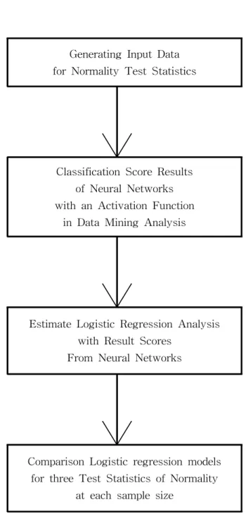
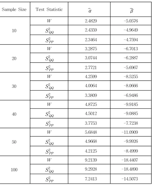
Figure 2 explains procedures briefly. Table 1 is summarized the estimated parameters in the logistic regression models by neural networks scores for each test statistics. In this table, we have estimated parameters, α and β, for several sample sizes such as size=10, 20, 30, 40, 50 and 100. We evaluate the performance of each test statistic for normality using the estimated slope of logistic regression model, β(Table 1). That is, the larger the absolute value of β, the better performance of corresponding test statistic. For example, in sample size 10, values of β s for three test statistics, W, S2QQ, and S2PP, are -5.0576, -4.9649, and -4.7594 respectively. Differences between β s of three statistics are small. The maximum value of these differences is 5.0576-4.7594=0.2982 and the minimum value is 5.0576-4.9649=0.0927. So we may say three normality statistics W, S2QQ, and S2PP are comparative for small sample n=10. But W and S2QQ statistic is superior to S2PP for other large samples.
Generating Input Data for Normality Test Statistics
Classification Score Results of Neural Networks with an Activation Function
in Data Mining Analysis
Estimate Logistic Regression Analysis with Result Scores
From Neural Networks
Comparison Logistic regression models for three Test Statistics of Normality
at each sample size
Figure 2. Framework for logistic regression analysis by classification of neural networks
Table 1 Estimation of parameters in logistic regression model
Sample Size Test Statistic α β
10
W 2.4829 -5.0576
S2QQ 2.4359 -4.9649
S2PP 2.3464 -4.7594
20
W 3.2875 -6.7013
S2QQ 3.0744 -6.2887
S2PP 2.7721 -5.6967
30
W 4.2599 -8.5255
S2QQ 4.0064 -8.0666
S2PP 3.3809 -6.9486
40
W 4.8725 -9.9185
S2QQ 4.5012 -9.0885
S2PP 3.7753 -7.7238
50
W 5.6848 -11.0909
S2QQ 4.9668 -9.9926
S2PP 4.2125 -8.4999
100
W 9.2139 -18.4407
S2QQ 9.2928 -18.4890
S2PP 7.2413 -14.5073
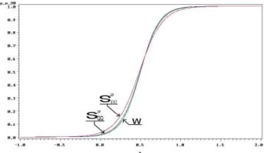
Figure 3 Estimation of logistic model at sample size=10
Figure 4 Estimation of logistic model at sample size=30
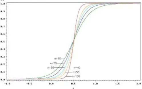
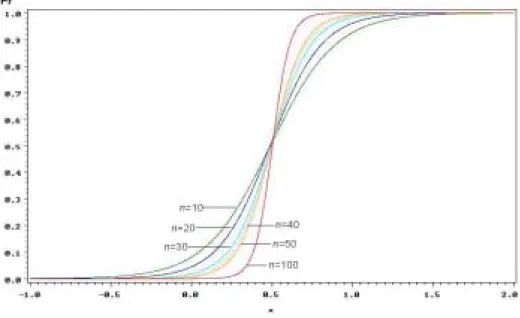
Through figures 3 and 4 of logistic regression models from (2.8), we compare the performance of these normality tests. The larger absolute value of β, the higher slope. Therefore the larger slope, the better performance. So, the figures of logistic regression models in Figure 3 are difficult to be distinguished the superior test statistic for small sample size 10. By the way, for sample size 30, values of βs for W, S2QQ, and S2PP, are -8.5255, -8.0666, and -6.9486 respectively. The maximum value of differences is 1.5769 between W and S2PP, the next grater value is 1.1180 between S2QQ and S2PP, and the minimum value is 0.4589 between W and S2QQ. So we can distinguish between W, S2QQ and S2PP. But it is still difficult to distinguish between W and S2QQ because of the small difference between β values of these two statistics in Figure 4. We conclude that W and S2QQ are comparative method for testing normality. Figure 5 shows graphs of logistic regression models for Shapiro-Wilk W statistic in various sample sizes, 10, 20, 30, 40, 50, and 100. According to increment of sample size, the slope of graph become higher. Figure 6 for test statistic S2QQ ( S2PP ) shows the same tendency as Figure 5.
Figure 5 Logistic regression for W at n =10, 20, 30, 40, 50 and 100
Figure 6 Logistic regression forS2QQ at n =10, 20, 30, 40, 50 and 100
4. Conclusions
The logistic regression model for normal and abnormal classifications is proposed by neural networks in data mining. By calculating sample variances of two normality graphical techniques(p-p and q-q plots), we tried goodness-of-fit comparison with numerical technique( Shapiro-Wilk statistic). Of course, it was possible by getting fitted logistic regression model, The results in Table 1, indicate that three normality statistics W, S2QQ, and S2PP are comparative for small sample n=10, but W and S2QQstatistics are superior to S2PP for other large samples. Through the Figures, we have similar results and conclusions.
5. References
1. Haykin, Simon (1999). Neural Network. Prentice Hall, New Jersey.
2. LaBrecque, J. (1977). Goodness-of-fit tests based on nonlinearity in probability plots, Technometrics. Vol. 19, 293-306.
3. Lee, J.-Y. and Rhee, S.-W. (1999). The Goodness-of-fit tests of normality by ROC curves, J of Information and Optimization Sciences, Vol. 20-3,
387-396.
4. Lee, J.-Y., Woo, J. S., and Rhee, S.-W. (1998). A transformed quantile-quantile plot for normal and bimodal distributions, J of Information and Optimization Sciences, Vol. 19-3, 305-318.
5. Mage, D. T. (1982). An objective graphical method for testing normal distributional assumptions using probability plots. The American Statistician, Vol. 36, 116-120.
6. Shapiro, S. S. and Wilk, M. B. (1965). An analysis-of-variance test for normality (complete sample), Biometrika, Vol. 52, 591-611.
7. Wilk, M. B. and Gnanadesikan, R. (1968). Probability plotting methods for the analysis of data, Biometrika, Vol. 55, 1-17.
[ received date : Dec. 2002, accepted date : Feb. 2002 ]