Journal of Institute of Control, Robotics and Systems (2015) 21(4):378-384
http://dx.doi.org/10.5302/J.ICROS.2015.14.0126 ISSN:1976-5622 eISSN:2233-4335
다중 인공신경망 기반의 실내 위치 추정 기법 Indoor Localization based on Multiple Neural Networks
손 인 수* (Insoo Sohn1,*)
1Division of Electronics & Electrical Engineering, Dongguk University - Seoul
Abstract: Indoor localization is becoming one of the most important technologies for smart mobile applications with different requirements from conventional outdoor location estimation algorithms. Fingerprinting location estimation techniques based on neural networks have gained increasing attention from academia due to their good generalization properties. In this paper, we propose a novel location estimation algorithm based on an ensemble of multiple neural networks. The neural network ensemble has drawn much attention in various areas where one neural network fails to resolve and classify the given data due to its' inaccuracy, incompleteness, and ambiguity. To the best of our knowledge, this work is the first to enhance the location estimation accuracy in indoor wireless environments based on a neural network ensemble using fingerprinting training data. To evaluate the effectiveness of our proposed location estimation method, we conduct the numerical experiments using the TGn channel model that was developed by the 802.11n task group for evaluating high capacity WLAN technologies in indoor environments with multiple transmit and multiple receive antennas. The numerical results show that the proposed method based on the NNE technique outperforms the conventional methods and achieves very accurate estimation results even in environments with a low number of APs.
Keywords: localization, location estimation, fingerprinting, neural network ensemble, IEEE 802.11n
I. INTRODUCTION
Location aware technology has become an important element for smart mobile devices, enabling services such as healthcare, personal navigation, and location-based marketing. Until recently, most of the localization research has been focused on outdoor environments based on global positioning system (GPS) technology. However, with the current trend toward increasing indoor wireless usage time, due to the proliferation of wireless local area networks (WLANs), the need for indoor localization technology is growing [1,2]. Unfortunately, the indoor location estimation is a very challenging problem for conventional outdoor localization methods that are based on GPS due to effects such as reflections, diffractions, and scattering due to number and type of objects between the indoor transmitters and receivers and resulted in problems such as poor indoor coverage, low accuracy, specialized hardware requirements [3-7].
To overcome the limitations of the GPS based outdoor localization technologies in indoor environments, various solutions targeted for indoor localization have been proposed. An overview of the commercial technologies for localization in wireless indoor systems can be found in [8]. The fingerprinting method based on the received signal strength (RSS) information is the most popular method in indoor WLAN environments due to the simplicity in RSS measurement collection process [9-11]. One of the most popular fingerprinting localization method is RADAR method based on the RSS information and K-nearest neighbor (KNN) algorithm proposed in [12] due to its simplicity. The RSS serves as the unique pattern feature corresponding to a position in
an indoor environment. Therefore, a database called radio map is constructed that contains RSS information of known reference points from different access points (APs) during the offline stage.
During the online stage, the location is estimated by averaging R reference points with the shortest signal space between the observed and stored RSS values. Another popular fingerprinting method is the area based probability (ABP) method [13]. Based on the radio map, ABP calculates the user location probability at all the reference points or areas and returns the area with the highest probability. Furthermore, authors in [14], proposed to reduce the RSS variation by averaging the effect of small-scale fading through the use of multiple antennas and, thus, improving the indoor localization performance. The impact of multiple antenna usage for localization was evaluated by analyzing various popular algorithms such as RADAR [12], area based probability (ABP) [13], and Bayesian network (BN) [15] under multiple antennas on an IEEE 802.11 testbed in a real office building.
Experimental results have shown that the multiple antenna based location estimation methods reduce the location estimation error up to 70% and improve the localization stability up to 100%
compared to the single antenna case.
Unfortunately, the RSS based signature pattern map that characterizes a user's location is highly nonlinear and may result in large location estimation error for certain locations [13,16]. To overcome this challenge, various artificial neural networks (NNs) based indoor localization solutions have been proposed due to the NN's good generalization properties with flexible modeling and learning capabilities. The multilayer perceptron neural network (MLPNN) [17] is a traditionally popular neural network and was first applied for outdoor code division multiple access (CDMA) mobile subscriber location estimation in [18]. This scheme uses the MLPNN with one input layer, two hidden layers, and an output layer structure as a parallel data fuser based on time of Copyright© ICROS 2015
* Corresponding Author
Manuscript received November 28, 2014 / revised January 2, 2015 / accepted January 27, 2015
손인수: 동국대학교 전자전기공학부([email protected])
arrival (TOA), direction of arrival (DOA), time difference of arrival (TDOA), and their confidence information. Another approach in [19] also used the MLPNN as a network-based outdoor mobile location estimation technique, but based on radio signal strength. Indoor fingerprinting algorithm based on MLPNN was proposed in [20] based on channel impulse response characteristics achieving distance location accuracy of 2 meters for 80% probability range. The radial basis function neural network (RBFNN) is another popular NN that was introduced in 1988 as a multivariate interpolator [21] and due to its simple network structure and computational complexity, it has been applied to many areas such as image processing, equalization, and localization. In [22], outdoor mobile user localization is performed by utilizing the RBFNN. The proposed RBFNN based estimator employs the RSS and the DOA as the input data to achieve location estimation error value of less than 100 meters in 80 percent probability range. Authors in [23] proposed the RBFNN based location estimation method for indoor wireless WLAN environments. The proposed RBFNN based technique was shown to be less complex and easier to train compared to the MLPNN based techniques. Furthermore, the RBFNN estimator achieved localization performance of median error equal to 3 meters.
One disadvantage of the NN based location estimation methods is that the performance is very dependent on the amount of training data available to the system and may result in poor localization accuracy in indoor environments with small number of APs resulting in insufficient amount of location data for successful NN configurations. Neural network ensemble (NNE), which is one of the emerging key technologies in the field of neural networks, [24-26] has drawn much attention in various areas where one neural network fails to resolve and classify the given data due to its' inaccuracy, incompleteness, and ambiguity.
The NNE overcomes this problem by combining a set of neural networks that learn to decompose a complex problem into simple sub-problems and then solve them efficiently. By combining multiple neural network outputs, the ensemble of neural network provides improved performance through collective decision rule compared to single neural network decision output. To improve the generalization capability and the location estimation performance of the conventional NN based fingerprinting location estimation methods, we propose a novel method based on ensemble of NNs. To evaluate the effectiveness of our proposed location estimation method, we conduct the numerical experiments using the TGn channel model [27] that was developed by the 802.11n [28, 29] task group for evaluating high capacity WLAN technologies in indoor environments with multiple transmit and multiple receive antennas. The experimental results show our proposed location estimation algorithm based on the NNE technique outperforms the conventional KNN and NN based algorithms in indoor wireless environments with single and multiple antennas.
The remainder of the paper is organized as follows. Section 2 provides an overview of the IEEE 802.11 TGn Model as well as our simulation methodologies. In section 3, we describe our proposed localization algorithm based on single NN and multiple NNs techniques. The experimental results are presented in section 4. Finally, conclusions are given in Section 5.
II. CHANNEL MODEL 1. Model Implementation
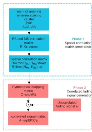
To simulate the IEEE 802.11 TGn compliant channel model, the MATLAB channel simulator [30] developed by Schumacher and Dijkstra was applied as part of the simulation platform to generate MIMO channel matrix. Based on the initial indoor scenario parameter settings, MIMO channel matrix H for channel profiles A to F can be easily generated. The TGn MIMO channel matrix is generated in two phase procedure as shown in Fig. 1. In the first phase, a spatial correlation matrix is generated for all the MSs and APs based on the number of antennas, antenna spacing, number of clusters, PAS, AS, and AoA. Based on the generated MS and AP spatial correlation matrices, the uplink or downlink spatial correlation matrices are generated by Kronecker product operations. In the second phase, the power delay profile is defined as the time dispersion of the non-line-of-sight and line-of-sight components with power coefficients. Finally, the MIMO channel matrix is created using fading signals derived from various Doppler spectra and power delay profiles and a from various Doppler spectra and power delay profiles and a symmetrical mapping matrix based on the spatial correlation matrix generated in the first phase. For channel profiles D and E, fluorescent light effect is added to the generated MIMO channel matrix.
2. Simulation Model
In our simulation model, we consider 50 m ´ 30 m rectangular field as our experimental testbed as shown in Fig. 2. There are 4 APs acting as RSS measurement devices for the radio signal transmitted by different MSs in various positions. The locations of all the APs are shown as blue star in Fig. 2 located at (10 m, 10 m), (40 m, 10 m), (10 m, 20 m), and (40 m, 20 m). There are R = 1500 reference points used as location estimation testing spots, located
그림 1. TGN MIMO 채널 매트릭스 생성 블록도.
Fig. 1. TGn MIMO channel matrix generation procedure.
손 인 수 380
uniformly with 1m separation from each other. The reference points are shown as black dots. The detailed steps of the simulation procedure are given as follows.
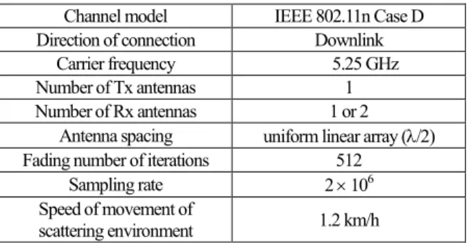
1) The TGn MATLAB channel simulator is configured to generate realizations of the channel matrices between the R reference points and 4 APs, where the reference points and APs are assumed to be the receiver side and transmitter side, respectively. The configuration parameters are shown in Table 1.
2) The generated channel matrices are processed by our MATLAB based module to calculate the received power of each spatial stream at the R reference points and obtain the mean SNR values as follows
2 2
,
1 1 1 1
( , ) / ,
T F M N
n m
i j m n
h i j
SNR TF
s
= = = =
æ ö
ç ÷
è ø
=
åå åå
(1)
where s2 is the Gaussian noise variance, M is the number of transmit antennas, N is the number of receive antennas, F is the number of subcarriers, and T is the number of symbols.
3) The received SNR values calculated in step 2 are collected and processed to construct the radio map of the experimental testbed based on fingerprint vector Sp=[SNRp1,SNRp2,
,SNRpK],
L for each reference point p, where K is the number of APs.
4) The test channel matrix is generated following the same procedure as in step 1.
Algorithm 1 RBF Neural Network based Location Estimation Algorithm 1: Initialization:
2: Construct fingerprint based InputTrainSeq from radio map.
3: Construct user location based DesOutputTrainSeq from radio map.
4: Normalize the training data by using mapminmax ( ).
5: Compute RBFcenterC using Eq. (3).
6: Randomly select G RBF centers from RBFcenterC.
7: end initialization 8:
9: while estimation error > threshold do 10: for i = 1 : G
11: Compute RBF output F(InputTrainSeq, RBFcenterC ).
12: end for
13: Compute RBFNN output (x_est, y_est) using Eq. (2).
14: Compute estimation error using diff((x_est, y_est), DesOutputTrainSeq).
15: Update weights w using LMS algorithm.
16: end while
그림 3. 알고리즘 1.
Fig. 3. Algorithm 1.
5) The proposed algorithm is evaluated based on the test channel matrix and the radio map constructed in step 3.
III. NEURAL NETWORK BASED FINGERPRINTING LOCALIZATION
1. Neural Network based Localization
Among various pattern matching methods, NN is one of the most popular methods due to the robustness against noise and interference with good generalization properties. The NN consists of interconnected neurons, which are adapted through a learning process to produce a desired pattern matching results. The neurons are grouped into three basic layers: the input layer, the hidden layer, and the output layer. The input layer is fed with input data and is processed in the hidden layer with appropriate activation functions. Each neuron in the hidden layer emits an output, which is a nonlinear function of its activation, and is processed in the output layer, to produce an output similar to the desired output.
Among numerous NN architectures, we propose to use the RBFNN [31] due to its properties such as small network size, fast network convergence, and simple weight adjustment procedure.
The output of the RBFNN can be represented as
( )
1
( ) ,
G
i i
i
F
=
=
å
F -x w x c (2)
where x is the input data vector, ci denotes the basis function center of RBF neurons, || x- ci || is the Euclidean distance between the input data vector and the basis function center, G is the total number of RBFs, wi denotes the weights of the output layer, F (·) is the radial basis function. As for the weights in the output layer, wi = [wix, wiy], they are iteratively trained to produce the desired (x, y) location of the users using least mean square (LMS) learning rule. We assume Gaussian radial basis function for our RBFNN, defined as F(|| x - ci ||) = exp(-b || x - ci ||).
The RBFNN is applied in this paper as the core pattern matching algorithm for fingerprinting based location estimation system. The RBFNN based location estimation algorithm can be described with two phases. The first phase is data collection stage and the second phase is the configuration phase. In the data collection stage, a radio map is constructed based on the postdetection SNR data obtained at all R reference points. In the network configuration stage, the radio map provides the required training input data to the RBFNN. The number of center units is set to be G < R, where R is the number of reference points.
Furthermore, the RBF centers are set equal to the mean value of
0 10 20 30 40 50
0 10 20 30
position y, m
position x, m
AP1 AP2
AP3 AP4
그림 2. 위치 추정 테스트베드 모델.
Fig. 2. Localization testbed model.
표 1. TGn 매트랩 채널 시뮬레이터 파라미터.
Table 1. TGn MATLAB channel simulator parameters.
Channel model IEEE 802.11n Case D Direction of connection Downlink
Carrier frequency 5.25 GHz
Number of Tx antennas 1
Number of Rx antennas 1 or 2
Antenna spacing uniform linear array (l/2) Fading number of iterations 512
Sampling rate 2 ´ 106
Speed of movement of
scattering environment 1.2 km/h
Ntr samples of fingerprint vectors at each reference points p expressed as
1
1 ,
Ntr
i pj
tr j
c S
N =
=
å
(3)where i = 1 … G and Spj is the fingerprinting vector for jth RSS sample. The detailed RBFNN based localization algorithm’s process is described in detail in Alg. 1. Before training the RBFNN, the training input and desired data are normalized by using the MATLAB function mapminmax. After the normalization, the scaled training data will fall in the range [-1, +1]. The reason for the normalization is that by mapping the training data values to [-1, +1], the RBFNN is able to converge faster with performance improvement.
2. Neural Network Ensemble based Localization
The NNE is a popular pattern matching method for problems with many local minima. By combining multiple neural network outputs, the ensemble of neural network provides improved performance through collective decision rule compared to single neural network decision output. The individual NNs are trained independently and the NNs are combined by majority or by weighted average method. The different weights correspond to different ways of forming generalization about the pattern given as the training set to each NN. In our proposed location estimation method, the weights are recomputed each time the NNE output is evaluated for best decision results for that particular instance. The output of NNE is a weighted average of all member neural networks’ output with the ensemble weights determined as a function of the relative error of each network. The general NNE output is defined as
( )
1
( ) ,
L i i i
F a f
=
=
å
x x (4)
where L is the number of neural network members in the ensemble, ai denotes the ensemble weights chosen to minimize the ensemble mean square error (MSE), and fi (x) is the i th neural network decision output. The proposed NNE based localization method is configured in three phases: the data collection phase, the network configuration phase, and the combination phase. The data collection phase and the network configuration phase are carried out to train the member NNs and are processed as described in the previous section. As for the combination stage, L NN output is combined to produce improved location estimation results. Two important factors in NNE construction are member network training and combination. In [32], various combination methods for ensemble of RBF networks were extensively studied
and LMS method was proven to be one of the best performing methods. Based on this study, the ensemble weight is trained by using LMS algorithm expressed as
( )
1 ( ),
k+ = k+d Fk-dk k
w w f x (5)
where d is the learning rate, Fk is the NNE output, dk denotes the desired location coordinates, and f (xk) is the output vector from member networks. The detailed NNE based localization algorithm’s process is described in detail in Alg. 2.
IV. NUMERICAL EVALUATIONS
The experimental testbed with dimension of 50m ´ 30m shown in Fig. 2 is used to analyze the performance of the proposed algorithm. The IEEE 802.11 TGn channel model profile D with mobile speed of 1.2 km/h, carrier frequency of 5.25 GHz, and signal bandwidth of 20 MHz was used. We collected postdetection SNR data at R = 1500 reference points from all 4 APs located as shown in Fig. 2. For each reference points, we collected 100 signal strength samples for training and testing purposes. From the collected 100 signal strength samples, 50 samples have been employed as training data samples to train the network and other 50 samples have been used as the testing data samples to test the proposed system with the corresponding user locations. The distance error is utilized as the main performance metric, which is a Euclidean distance between the estimated location and the true location of the user to be localized.
Based on the radio map constructed in the data collection stage, each member RBFNN is trained in the network configuration stage by setting the number of center units to G = 100, RBF centers equal to Ntr = 50 samples of fingerprint (FP) vector, and the number of training iteration to 50000 with learning rate equal d to 0.001. In the NNE combination stage, two member RBFNN output is combined based on the ensemble weights that were obtained through LMS algorithm with the number of training iteration equal to 10000 with learning rate set to 0.0001. Fig. 5 shows the CDF of the localization error for the proposed NNE method, RBF method with single network, MLP method with one input layer and two hidden layers, and the traditionally popular
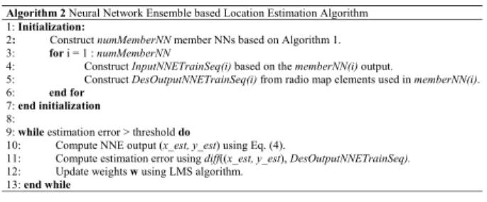
Algorithm 2 Neural Network Ensemble based Location Estimation Algorithm 1: Initialization:
2: Construct numMemberNN member NNs based on Algorithm 1.
3: for i = 1 : numMemberNN
4: Construct InputNNETrainSeq(i) based on the memberNN(i) output.
5: Construct DesOutputNNETrainSeq(i) from radio map elements used in memberNN(i).
6: end for 7: end initialization 8:
9: while estimation error > threshold do
10: Compute NNE output (x_est, y_est) using Eq. (4).
11: Compute estimation error using diff((x_est, y_est), DesOutputNNETrainSeq).
12: Update weights w using LMS algorithm.
13: end while
그림 4. 알고리즘 2.
Fig. 4. Algorithm 2.
0 1 2 3 4 5 6 7 8 9 10 11 12 13 14 15
0.0 0.1 0.2 0.3 0.4 0.5 0.6 0.7 0.8 0.9 1.0
cumulative distribution function (CDF)
error distance (m)
NNE RBF MLP KNN
그림 5. NNE, RBF, MLP 및 KNN 기법에 따른 오류 거리 CDF 그래프.
Fig. 5. Error distance CDF performance for NNE, RBF, MLP, and KNN localization methods.
손 인 수 382
KNN method. The number of member networks is equal to L = 2 which were trained independently with first network based on the FP data corresponding to APs positioned at (10 m, 10 m) and (40 m, 10 m). Furthermore, the second network was trained with data from APs at (10 m, 20 m) and (40 m, 20 m). As shown in the figure, the neural network based algorithms outperform the KNN method significantly. Furthermore, we can observe that by combining two neural network outputs trained by different AP RSS data, the proposed algorithm improves the localization performance compared to one RBF method and outperforms the MLP method.
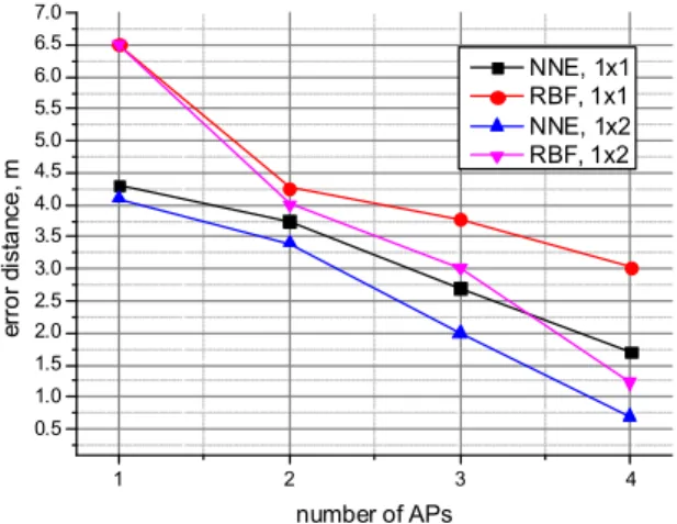
To evaluate the performance of the NNE based localization system with multiple antennas, each RBF member network is configured by setting the number of center units to G = 50, RBF centers equal to Ntr = 50 samples of fingerprint vector, and the number of training iteration to 5000 with learning rate equal d to 0.05. Note that the RBF centers are randomly chosen from R = 1500 reference points. Fig. 6 illustrates the CDF of the localization error for the proposed NNE and the RBF methods with 1´1 and 1´2 antenna configurations. One can observe that for both schemes, the increase in the number of receive antennas effectively improves the performance. Furthermore, we discover that the performance improvement due to the proposed method is decreased in multiple antenna scenario compared to the single antenna case. The results demonstrate that further performance gain is difficult to achieve in addition to the performance gain due to the multiple antenna diversity gain. The CDF of the localization error for the NNE and RBF method with 1´1 and 1´2 antenna configurations is depicted in Fig. 7 with different number of APs.
For Four AP environment, the number of member networks is set to L = 2, trained independently, with AP1 and AP2 FP data assigned to the first member network and AP3 and AP4 FP data assigned to the second member network. For the 3 AP case, AP1 and AP2 FP data were assigned to the first member network and AP3 FP data was assigned to the second member network. In the case of 2 APs, AP1 FP data was assigned to the first member network and AP2 FP data to the second member network. For one AP case, to obtain two different training data sets for two
independent member networks construction, the order of the AP FP data samples were randomly shifted for all the member networks. From the results shown in the figure, we can see that compared to the RBF method, the NNE method achieves better performance for number of APs equal to 3 and 4. However for two AP case, the numerical results show small NNE performance improvement compared to three and four AP results. This is due to the similar architecture of the NNE compared to the RBF algorithm. Two different one dimensional data assigned to two network based NNE provides small increase in the available degree of information compared to two dimensional data assigned to a single network. However, note that for one AP case, by applying independently trained data to each member network of NNE, the proposed method does gain superior performance improvement with very low median error values less than 4.5 m for both single and double antenna cases. Furthermore the figure shows with increase in the number of receive antennas, large performance improvement is observed. However, as the number of APs is decreased, the multiple antennas' effectiveness is reduced due to the degradation in the RBF network's nonlinear mapping function.
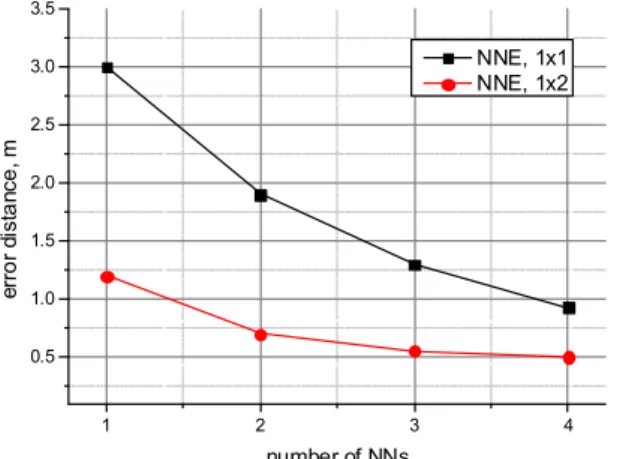
In order to study the performance impact with respect to the number of member networks, we compare the location estimation accuracy results in Fig. 8. The number of APs is fixed to four as shown in Fig. 2. For one and two member network based NNE systems, same configuration was used as in the previous experiments. For three member network NNE, AP1 and AP2 FP data were assigned to the first member network, AP3 FP data was assigned to the second member network, and AP4 FP data was assigned to the third network. For four member network NNE, both AP1 and AP2 FP data were assigned to the first and third member networks and both AP3 and AP4 FP data were assigned to the second and fourth member networks providing two dimensional data to each member network. As the number of member network is increased from one to two, enhanced estimation accuracy is observed in Fig. 8. However, as the number of member network is increased to three and four, the improvement is decreased due to the reduced available degree of information provided to the member networks.
0 1 2 3 4 5 6 7 8 9 10 11 12 13 14 15
0.0 0.1 0.2 0.3 0.4 0.5 0.6 0.7 0.8 0.9 1.0
cumulative distribution function, CDF
error distance, m
NNE, 1x1 RBF, 1x1 NNE, 1x2 RBF, 1x2
그림 6. 다중 안테나 기반의 NNE 및 RBF 기법에 따른 오류 거리 CDF 그래프.
Fig. 6. Error distance CDF performance with different antenna configurations for NNE and RBF methods.
1 2 3 4
0.5 1.0 1.5 2.0 2.5 3.0 3.5 4.0 4.5 5.0 5.5 6.0 6.5 7.0
error distance, m
number of APs
NNE, 1x1 RBF, 1x1 NNE, 1x2 RBF, 1x2
그림 7. 엑세스 포인트 수에 따른 다중 안테나 기반의 NNE 및 RBF 기법의 오류 거리 성능 그래프.
Fig. 7. Error distance performance with different number of APs and multiple antennas for CDF = 0.5.
Insoo Sohn
1 2 3 4 0.5
1.0 1.5 2.0 2.5 3.0 3.5
error distance, m
number of NNs
NNE, 1x1 NNE, 1x2
그림 8. 다양한 인공신경망 수에 따른 다중 안테나 기반의 NNE 및 RBF 기법의 오류 거리 성능 그래프.
Fig. 8. Error distance performance with different number of NNs and multiple antennas for CDF = 0.5.
V. CONCLUSIONS
In this paper, we propose a novel location estimation algorithm based on NNE. To the best of our knowledge, this is the first time that NNE technique has been applied in the area of indoor wireless location estimation problem. The proposed NNE based algorithm is based on multiple NNs that are trained independently using a database called radio map containing RSS information from multiple APs. We evaluate the proposed algorithm by investigating the resulting cumulative distribution function respect to the error distance estimation using the TGn channel model that was developed by the IEEE 802.11n task group with multiple transmit and receive antennas. The experimental results indicate that our approach achieves significant improvements of the location estimation accuracy compared to the conventional methods with single and multiple antennas. Furthermore, the numerical results show that the proposed algorithm achieves a very low location estimation error even in indoor wireless environments with only single AP, which was not possible previously with conventional methods.
REFERENCES
[1] K. Pahlavan, X. Li, and J. Makela, “Indoor geolocation science and technology,” IEEE Communications Magazine, vol. 40, no.
2, pp. 112-118, 2002.
[2] H. Liu, H. Darabi, P. Banerjee, and P. Liu, “Survey of wireless indoor positioning techniques and systems,” IEEE Transactions on Systems, Man, and Cybernetics, vol. 37, no. 6, pp. 1067-1080, 2007.
[3] S. Tekinay, “Wireless geolocation systems and services,” IEEE Communications Magazine, vol. 36, no. 5, p. 28, 1998.
[4] A. H. Sayed, A. Tarighat, and N. Khajehnouri, “Network-based wireless location: Challenges faced in developing techniques for accurate wireless location information,” IEEE Signal Processing Magazine, vol. 22, no. 4, pp. 24-40, 2005.
[5] H. Akcan and C. Evrendilek, “GPS-free directional localization via dual wireless radios,” Computer Communications, vol. 35, no. 9, pp. 1151-1163, 2012.
[6] P. Almers, E. Bonek, and A. Burr, et al., “Survey of channel and radio propagation models for wireless MIMO systems,”
EURASIP Journal on Wireless Communications and Networking, vol. 2007, pp. 1-20, 2007.
[7] H.-M. Lee and D.-S. Kim, “Insect-inspired algorithm for zone radius determination of ad-hoc networks,” Journal of Institute of Control, Robotics, and Systems (in Korean), vol. 20, no. 10, pp.
1079-1083, 2014.
[8] Y. Gu, A. Lo, and I. Niemegeers, “A survey of indoor positioning systems for wireless personal networks,” IEEE Communications Surveys & Tutorials, vol. 11, no. 1, pp. 13-32, 2009.
[9] T. Roos, P. Myllymaki, H. Tirri, P. Misikangas, and J. Sievanen,
“A probabilistic approach to WLAN user location estimation,”
International Journal of Wireless Information Networks, vol. 9, no. 3, pp. 155-164, 2002.
[10] G. Deak, K. Curran, and J. Condell, “A survey of active and passive indoor localisation systems,” Computer Communica- tions, vol. 35, no. 16, pp. 1939-1954, 2012.
[11] S. Y. Cho and J. G. Park, “Radio propagation model an spatial correlation method-based efficient database construction for positioning fingerprints,” Journal of Institute of Control, Robotics, and Systems (in Korean), vol. 20, no. 7, pp. 774-781, 2014.
[12] P. Bahl and V. N. Padmanabhan, “RADAR: An in-building RF- based user location and tracking system,” Proc. of the IEEE INFOCOM, pp. 775-784, Mar. 2000.
[13] E. Elnahrawy, X. Li, and R. P. Martin, “The limits of localization using signal strength: a comparative study,” Proc. of the IEEE SECON, pp. 406-414, Oct. 2004.
[14] K. Kleisouris, Y. Chen, J. Yang, and R. P. Martin, “Empirical evaluation of wireless localization when using multiple antennas,” IEEE Trans. Parallel and Distributed Systems, vol.
21, no. 11, pp. 1595-1610, 2010.
[15] D. Madigan, E. Elnahrawy, R. P. Martin, W. Ju, P. Krishnan, and A. Krishnakumar, “Bayesian indoor positioning systems,”
Proceeding of the IEEE INFOCOM, pp. 1217-1227, Mar. 2005.
[16] G. Chandarasekaran, M. Ergin, J. Yang, S. Liu, Y. Chen, M.
Gruteser, and R. Martin, “Empirical evaluation of the limits on localization using signal strength,” Proc. of the IEEE SECON, pp. 1-9, Jun. 2009.
[17] S. Haykin, Neural Networks, A Comprehensive Foundation, Macmillan, 1994.
[18] S. Merigeault, M. Batariere, and J. N. Patillon, “Data fusion based on neural network for the mobile subscriber location,”
Proc. of the IEEE VTC, pp. 536-541, Sep. 2000.
[19] H. Zamiri-Jafarian, M. M. Mirsalehi, I. Ahadi-Akhlaghi, and H.
Keshavarz, “A neural network-based mobile positioning with hierarchical structure,” Proc. of the IEEE VTC, pp. 2003-2007, Apr. 2003.
[20] C. Nerguizian, C. Despins, S. Affes, G. I. Wassi, and D. Grenier,
“Neural network and fingerprinting-based geolocation on time- varying channels,” Proc. of the IEEE PIMRC, pp. 1-6, Sep.
2006.
[21] D. S. Broomhead and D. Lowe, “Multivariable functional interpolation and adaptive networks,” Complex Syst., vol. 2, pp.
321-355, 1988.
[22] H. Zamiri-Jafarian, M. M. Mirsalehi, I. Ahadi-Akhlaghi, and K.
N. Plataniotis, “Mobile station positioning using radial basis function networks,” Proc. of the IEEE PIMRC, pp. 2797-2800,
손 인 수 384
Sep. 2004.
[23] C. Laoudis, P. Kemppi, and C. G. Panayiotou, “Localization using radial basis function networks and signal strength fingerprints in WLAN,” Proc. of the IEEE GLOBECOM, pp. 1- 6, Nov. 2009.
[24] L. K. Hansen and P. Salamon, “Neural network ensembles,”
IEEE Trans. Pattern Analysis and Machine Intelligence, vol. 12, no. 10, pp. 993-1001, 1990.
[25] A. Krogh and J. Vedelsby, “Neural network ensembles, cross validation, and active learning,” Advances in Neural Information Processing Systems 7, pp. 231-238, 1995.
[26] D. Jimenez, “Dynamically weighted ensemble neural network for classification,” Proc. of the IEEE World Congress on Computational Intelligence, vol. 1, pp. 753-756, Jul. 1998.
[27] TGn Channel Models, IEEE Std. 802.11-03/940r4, May 2004.
[28] E. Perahia, “IEEE 802.11n development: history, process, and technology,” IEEE Commun. Mag., vol. 46, no. 7, pp. 48-55, 2008.
[29] T. K. Paul and T. Ogunfunmi, “Wireless LAN comes of age:
understanding the IEEE 802.11n amendment,” IEEE Circuits and Systems Mag., vol. 8, no. 1, pp. 28-54, 2008.
[30] L. Schumacher and B. Kijkstra, Description of a MATLAB Implementation of the Indoor MIMO WLAN Channel Model Proposed by the IEEE 802.11 TGn, May 2004.
[31] I. Sohn and N. Ansari, “Configuring RBF neural networks,”
Electronics Letters, vol. 34, no. 7, pp. 684-685, 1998.
[32] J. Torres-Sospedra, C. Hernandez-Espinosa, and M. Fernandez- Redondo, “A comparison of combination methods for ensembles of RBF networks,” Proc. of the IEEE IJCNN, pp.
1137-1141, Jul.-Aug. 2005.
손 인 수
1994년 RPI 컴퓨터공학과 졸업. 1996년 NJIT 공학석사. 1998년 SMU 공학박사.
1998년 에릭슨 달라스 선임연구원. 1999 년~2004년 한국전자통신연구원 선임연 구원. 2004년~2006년 명지대학교 통신공 학과 조교수. 2006년~현재 동국대학교 전자전기공학부 부교수. 관심분야는 통신신호처리, 기계학습, 게임이론, 그린통신 등.