Active Random Noise Control using Adaptive Learning Rate Neural Networks

(1)

ICCAS2005 June 2-5, KINTEX, Gyeonggi-Do, Korea

1. INTRODUCTION

This paper presents an active random noise control using adaptive learning rate neural networks. In recent years, many researchers have reported on the active noise control. A wide range different types of dependence on time of the signals observed occur in acoustical and vibration problems. These can range from the perfectly predictable continuous sinusoidal pressure fluctuation to a random fluctuation with time whose value at any instant is in practice unpredictable from knowledge of its previous values. These two types of signal represent two broad classes of fluctuation which are generally termed either “deterministic” or “random”. Random fluctuations are those whose values cannot be predicted perfectly from the previous time history.

Adaptive linear filtering techniques have been extensively used for the active control of sound and vibration, and many of today’s implementations of active control use those techniques. A popular adaptive filtering algorithm is the multi channel filtered-X LMS algorithm because of its simplicity and it’s relatively low computational load. This algorithm is a steepest descent algorithm that uses an instantaneous estimate of the gradient of the cost function. This algorithm uses adaptive FIR filters for the digital controller. However, such filters typically require fewer coefficients, but the convergence is not as predictable as in the case of adaptive FIR filters. The topic of artificial NN (ANN) for identification and control is at present one of the key research areas in the field of control systems. ANN has been proposed by information and neural science as a result of the study of the mechanisms and structures of the brain. This has led to the development of new computational models, based on this biological back-ground, for solving complex problems like pattern recognition, fast information processing, learning and adaptation.

If the learning rate is too large, then the NN can over-shoot the minimum cost value, jumping back and forth over the minimum and failing to converge. Moreover, it can be shown that the learning rate in a layer must decrease as the number of neurons in that layer increases. Aside from correcting these problems, adapting the learning rate can significantly speed up the convergence of the weights. The adaptive learning rate strategy increases the learning rate by a small constant if the current partial derivative of the objective function with respect to the weight and the exponential average of the previous

derivatives have the same sign, otherwise the learning rate is decreased by a proportion of its value. The use of an adaptive learning rate attempts to keep the learning step size as large as possible without leading to oscillation. It is expected that a cost function minimize rapidly and training time is decreased.

This paper will focus on the problem of active random noise control using adaptive learning rate Neural Networks. Numerical simulations and experiments of active random noise control with the transfer function of the error path will be performed, to validate the convergence properties of the adaptive learning rate Neural Networks. Control results show that adaptive learning rate Neural Networks control structure can outperform linear controllers and conventional neural network controller for the active random noise control.

2. ACTIVE NOISE CONTROL

Controller Primary source Mic . Primary path Secondary path Speaker Mic . Quiet zone ･ Control point Secondary source Controller Primary source Mic . Primary path Secondary path Speaker Mic . Quiet zone ･ Control point Secondary source

Fig. 1 Schematic diagram of an active noise control system. The concept of active sound control has been presented by Lueg’s original patent in 1936. Active sound control works on the principle of destructive interference between an original “primary” disturbance sound field and a “secondary” sound field that is generated by some control actuators. Fig. 1 shows a schematic diagram of an active noise control system with an actuator and two sensors (a loudspeaker and two microphones in this case). A left side microphone (called a reference sensor) is used to measure an advanced information on the disturbance sound wave, and right side microphone (called an error sensor) is used to monitor the performance of the active

Active Random Noise Control using Adaptive Learning Rate Neural Networks

Minoru Sasaki*_{, Takumi Kuribayashi}**_{, and Satoshi Ito}***

* ** *** _{Department of Human and Information Systems Engineering, Gifu University, Gifu, Japan}

*_{(Tel : +81-58-293-2541; E-mail: [email protected])} **_{(Tel : +81-58-293-2542; E-mail: [email protected])}

***_{(Tel : +81-58-293-2540; E-mail: [email protected])}

Abstract: In this paper an active random noise control using adaptive learning rate neural networks is presented. The adaptive learning rate strategy increases the learning rate by a small constant if the current partial derivative of the objective function with respect to the weight and the exponential average of the previous derivatives have the same sign, otherwise the learning rate is decreased by a proportion of its value. The use of an adaptive learning rate attempts to keep the learning step size as large as possible without leading to oscillation. It is expected that a cost function minimize rapidly and training time is decreased. Numerical simulations and experiments of active random noise control with the transfer function of the error path will be performed, to validate the convergence properties of the adaptive learning rate Neural Networks. Control results show that adaptive learning rate Neural Networks control structure can outperform linear controllers and conventional neural network controller for the active random noise control.

(2)

sound control system, thus providing feedback to a control algorithm. The control structure of Fig. 1 is called feedforward, because the controller feeds the actuator with a signal based on the advanced information obtained from the reference sensor. If the controller works properly, the signal sent in the actuator will generate a sound wave that will cancel the disturbance sound wave at the location of the quiet zone. Detailed presentations of active sound control theory and applications can be found in [1-4].

Adaptive linear filtering techniques have been extensively used for the active control of sound and vibration, and many of today’s implementations of active control use those techniques. The filtered-x LMS algorithm is most widely accepted feedforward control algorithm because of its ease of implementation and remarkable performance. However, this algorithm has an inherent drawback because of the required control-to-error transfer function model. This model is typically obtained off-line and thus is not adaptive to changes in the control-to-error plant. An alternative algorithm, based on the gradient search using Newton’s method and termed the time-averaged gradient (TAG) algorithm, has been presented. The updated algorithm only requires input from the error signal. This algorithm is adaptive and does not require an off-line model of the plant. The linear digital controllers described may not perform well in the cases where nonlinearities and random processes are found in an active control system. The use of a nonlinear controller can improve the control performance on a system with a nonlinear and random behavior, and neural networks can be used as nonlinear controllers for such an active random noise control.

3. NEURAL ADAPTIVE NOIS E CONTROL SYSTEM

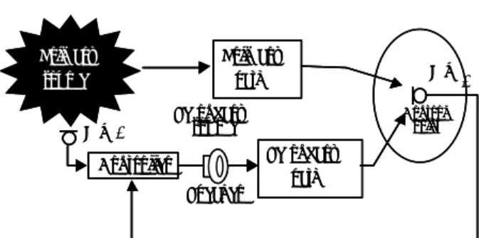
The block diagram of an active noise control system is shown in Fig. 2. A three layer neural networks is used for the active random noise control. The backpropagation method is used for learning rule of this system. The backpropagation learning rule is used to train nonlinear, multilayered networks to perform function approximation, pattern association, and pattern classification. The backpropagation method is a gradient descent method that establishes the weights in a multi-layer, feedforward adaptive neural network. Learning is accomplished by successively adjusting the weights based on a set of input patterns and a corresponding set of desired output patterns. During this iterative process, an input pattern is presented to the network and propagated forward to determine the resulting signal at the output units. The differences between the actual resulting output signal and the predetermined desired output signal in each output unit represents an error that is backpropagated through the network in order to adjust the weights. This error is computed as the sum of the root-mean squares of the difference between the actual and desired outputs at each output node. The learning process continues until this error is below a preset value over the entire set of input patterns. The training process using backpropagation is not an easy one. Backpropagation can be improved in two different ways: by heuristics, and by using more powerful methods of optimization. Momentum decreases backpropagation’s sensitivity to small details in the error surface. This helps the network avoid getting stuck in shallow minima which would prevent the network from finding a lower error solution.

The sound pressure signal of the noise taken in by the controller and its history are used for the input of a network.

The activation function of input layer and output layer is a

linear function, and one of a hidden layer is a sigmoid function. ï ï þ ï ï ý ü ÷ ÷ ø ö ç ç è æ + × = ÷÷ ø ö çç è æ + × =

å

j k j jk O k i i i ij H j y w f y y w f y g q

(1)

O k H j I iÎ Î Î

where I expresses a set of the index of the unit of the input layer. H expresses a set of the index of the unit of a hidden layer. O expresses a set of the index of the unit of the output layer, respectively. i is the number of the unit of an input layer.

j is the number of the unit of a middle layer. k is the number of

the unit of an output layer, respectively. yi is the output of an input layer. yj is the output of a hidden layer. yk is the output of an output layer. fH(*) is an output function in a hidden layer. fO(*) is an output function in a output layer. wij is the weight of between an input layer and a hidden layer. wjk is the weight of between a hidden layer and an output layer. qi is the bias of hidden layer. gk is the bias of output layer, respectively.

An cost function is expressed as

2 2 ₍ ₎ 2 1 2 1 i i j d y e E= = -

(2)

The learning rule and the updating equation of the weigh ts can be written as ) (n e y E k -= ¶ ¶

₍₃₎

( )

n e y n w f n e j k j jk o k = ÷ ÷ ø ö ç ç è æ + × ¢ × =

å

g d ( ) ( )

(4)

å

-+ × × × = ÷÷ ø ö çç è æ + × ¢ × × = k j j jk k k i j i ij H jk k j y y n w y n w f n w ) 1 )( 1 ( 2 1 ) ( ) ( ) ( e d q d s

(5)

) ( ) 1 (n w y w n w j jk k jk jk + = -a×d × -h×

(6)

k k k n g n b d g ( +1)= ( )- ×

(7)

) ( ) 1 (n w y w n w j _i _ij ij ij + = -a×s × -h×

(8)

j j j n q n b s q ( +1)= ( )- ×

(9)

where a is the learning rate that affects the convergence

speed and stability of the weights during learning, b is the

momentum constant, h is the learning rate of the bias.

(3)

units, a hidden layer with 10 units and an output layer with a

single unit.

Fig. 2 Active noise control system.

4. ADAPTIVE LEARNING RATE NNS The backpropagation method is a gradient descent method that establishes the weight in a multi-layer, feed-forward adaptive NN. Learning is accomplished by successively adjusting the weight based on a set of input patterns and a corresponding set of desired output patterns. During this iterative process, an input pattern is presented to the network and propagated forward to determine the resulting signal at the output units. The differences between the actual resulting output signal and the predetermined desired output signal in each output unit represents an error that is backpropagated through the network in order to adjust the weights. The learning process continues until the network responds with an output signal the sum of whose root-mean square errors from the desired output signals are less than a preset value. The training process using backpropagation is a difficult process. It is necessary to find an appropriate architecture, adequate size and quality of training data, satisfactory initialization, learning parameter values, and to avoid over-training effects. Several improvements can be made to correct deficiencies in gradient descent NN learning algorithms. These can be applied at each layer of a multilayer NN when using backpropagation tuning. Improvements in performance are given by using learning with momentum, using an adaptive learning rate, etc.

To speed up the convergence behavior, the selection of parameters such as the learning rates is done by using the utilization of a momentum factor. The learning rule utilized consists of a weight update using momentum b with the exception that each weight has its own learning rate parameter

a. To minimize the cost function E, the updating equation of

the weights is defined by the activation function of input layer and output layer is a linear function, and one of a hidden layer is a sigmoid function.

If the learning rate a is too large, then the NN can

overshoot the minimum cost value, jumping back and forth over the minimum and failing to converge.

Moreover, it can be shown that the learning rate in a layer must decrease as the number of neurons in that layer increases.

Aside from correcting these problems, adapting the learning rate can significantly speed up the convergence of the weights.

The adaptive learning rate strategy increases h by a small

constant if the current partial derivative of the objective function E with respect to the weight wjk and the exponential average of the previous derivatives have the same sign, otherwise h is decreased by a proportion of its value.

This IF-THEN algorithm is shown as follow,

1.

( ) ( ) ( )()

+ D

( )

-1 ¶ ¶ = D w t t w t E t t w ij ij ij h b If : E(t-1) < E(t)

then : retain wij (t+1) and increase learning step size,

h(t+1) = (1+f) h(t)

Go to 2.

Else if : E(t+1) > E(t)

then : reject wij (t+1) and decrease learning step size,

h(t+1) = (1-f) h(t)

Go to 1. 2. t=t+1

Go to next iteration.

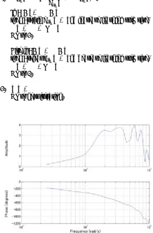
Fig. 3 Bode diagram of transfer function H.

5. SIMULATION RESULTS

The white noise after passing through a LPF for the random signal is used in the simulation as shown in Fig. 5. Cutoff frequency of the LPF is 1000Hz. Fig. 3 shows the acoustic transfer function substituted for the sound transfer system H of the block diagram as shown in Fig. 2. The gain characteristic and the phase characteristics of the acoustic transfer function is a transfer function from our lab’s data. This acoustic transfer function has two mechanical resonance frequencies in 300 Hz, 500 Hz, 800 Hz and 1200 Hz. Fig. 4 shows the noise signal for the simulation and the control result of the neural adaptive filter. Simulation conditions are shown in Table 1. Fig. 5 is the power spectrum of the noise signal and control result signal. Within 0.3 seconds the network decreases 80% of the random noise. Fig. 5 shows that the neural network can control whole noise frequency band from 0Hz to 1000Hz. The results of the simulation show that the H:Acoustic transfer function

C:Acoustic transfer function S(n):Input signal

d(n):Output signal e(n):Error signal

(4)

adaptive learning rate neural network controller provides effective alternatives to an active random noise control.

Fig. 4 Simulation result of adaptive learning method.

Fig. 5 FFT diagram of adaptive learning method.

Table 1 Simulation parameter of ALBP method.

Sampling Time 0.0001 sec

Simulation length 2 sec

Unit number of input layer 10 Unit number of hidden layer 10 Unit number of output layer 1 Weight correction parameter a 1×10-3

Offset correction parameter b 1×10-8 Moment parameter h 1×10-8

6. EXPERIMENTAL RESULTS

Some real-time control experiments of active random noise control were performed, in order to evaluate the performance of the adaptive learning rate neural network controller for an

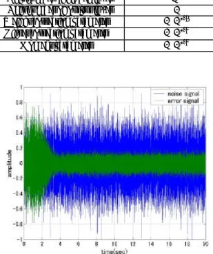
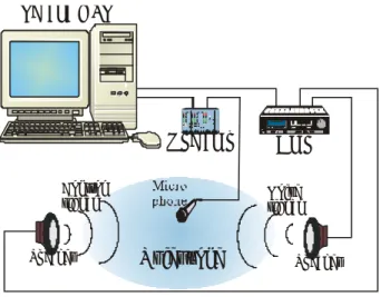
active random noise control. Fig. 8 shows the experimental setup, including two loudspeakers (BOSE Model 121), a microphone (SONY Model ECM-261), a power amplifier, a preamplifier, A/D and D/A converters, a PC and a DSP system (dSPACE Model DS1104). When the learning algorithm had converged to a good control solution or when a certain number of iterations of optimization had been performed, the solution of the controller was downloaded into the DSP system, where the forward propagation was computed in real-time for the control network. The white noise after passing through a BPF for the random signal is used in the experiment as shown in Fig. 7. Band pass frequency of the BPF is from 200Hz to 400Hz (6th_{order Butterworth band-pass filter) for the} limitation of the real-time computations by the DSP. Fig. 6 shows the noise signal for the experiment and the control result of the neural adaptive filter. In the experiment at first 2 seconds the controller was switched off. And then the controller was switched on. The experiment conditions are shown in Table 3. Fig. 7 is the power spectrum of the noise signal and control result signal. The adaptive rate learning neural network controller produced 70% reduction during the control stage. Fig. 9 shows the noise signal for the experiment and the control result of the conventional backpropagation neural adaptive filter. Fig. 10 is the power spectrum of the noise signal and control result signal of the conventional backpropagation neural network. The experiment conditions of the conventional backpropagation neural network are shown in Table 4. With comparison to the conventional backpropagation neural network method, the proposed adaptive learning rate neural network controller has a faster convergence speed and good control performance for the active random noise control.

Table 2 Experimental parameter of ALBP method.

Experimental length 20 sec

Offset correction parameter b 1×10-8

Moment parameter h 1×10-8

(5)

Fig. 7 FFT diagram of adaptive learning method.

Quiet zone

Speaker _Speaker

Ope amp

Amp

PC and DSP

Control

signal Noise_signal

Fig. 8 Experimental setup.

Fig. 9 Experimental results of conventional backpropagation method.

Fig. 10 FFT diagram of conventional backpropagation method.

Table.3 Experimental parameter of BP method.

Experimental length 20 sec

Offset correction parameter b 1×10-8

Moment parameter h 1×10-8

7. CONCLUSION

This paper presents an active random noise control using adaptive learning rate neural networks. Numerical simulations and experiments of active random noise control with an acoustic transfer function of the error path are performed to validate the convergence properties of the Neural Networks. Control results show that the adaptive learning rate neural networks controller can outperform the conventional backpropagation neural network controller for the active random noise control. Within 0.5 seconds the adaptive rate learning neural networks decreases 80% of the random noise. The results of the simulation and experiment show that the adaptive neural network controller provides effective alternatives to an active random noise control.

REFERENCES

[1] M. Nakamura, H. Hata, Y. Nakamura, T. Endo, and K. Iizuka, “Vibration Reduction in Rolling Piston-Type Compressors through Motor Torque Control(Basic Study on Theoretical Analysis and Computer Simulation),”

JSME International Journal, Series Ⅲ, Vol. 34, No. 2,

pp. 200-209, 1991.

[2] K. Seto, “Optimum Design Method of Active Dynamic Absorbers and Its Vibration Control Effect,” Proceedings

of International Symposium on Active Control of Sound and Vibration, pp. 79-98, 1991.

[3] M. Takahashi, R. Gtohda, T. Yamada, K. Asami, and H. Hashida, “Broadband Active Noise Control of Air-Conditioning Duct Systems in Auditoriums , ”

(6)

Control of Sound and Vibration, pp. 272-278, 1991.

[4] S. Suzuki, K. Nagayasu, T. Hay ashi, S. Saruta, H. Tamura, Y. Sakiguchi, and K. Nakanishi, “A Basic Study on an Active Noise Control System for Compressor Noise in a Refrigerator,” Proceedings of International

Symposium on Active Control of Sound and Vibration, pp.

255-260, 1991.

[5] S. Hasegawa, T. Tabata, A. Kinoshita, and H. Hyodo, “The Development of an Active Noise Control System for Automobiles ,” SAE Technical Paper Series, No. 922086, 1992

[6] Kido, “Active control of noise,” Acoustical Society of

Japan, Vol. 47, No. 9, pp. 661-667, 1991.

[7] H. Hort, ”Experiments in The Stabilization of Ships,”

STG, Vol. 35, 1934.

[8] P. Lueg, “Verfahren zur Dämpfung von Schallschwingungen,” German Patent No. 655, 508 Filed: Jan. 27, 1933. Patented: Dec. 30, 1937.

[9] W.B. Conover, ”Fighting Noise with Noise,” Noise

Control, Vol. 2, pp. 78-82, 1956.

[10] H.F. Olson, and E.G. May, “Electric Sound Absorber,”

Journal of The Acoustical Society of America, Vol. 25, pp.

1130-1136, 1953.

[11] M.A. Swinbanks, “The Active Control of Sound Propagation in Long Ducts,” Journal of Sound and

Vibration, Vol. 27, pp. 411-436, 1973.

[12] J.H.B. Poole, and H.G. Leventhall, “An Experimental Study of Swinbanks’ Method of Sound in Ducts, ”

Journal of Sound and Vibration, Vol. 49, pp. 257-266,

1976.

[13] C.F. Ross, “An Algorithm for Designing a Broadband Active Sound Control System,” Journal of Sound and

Vibration, Vol. 80, pp. 373-380, 1982.

[14] A. Rouse, “Self-adaptive Broadband Active Sound Control System,” Academic Press Inc., pp. 373-380, 1985.

[15] B. Widrow , and M.E. Hoff, “Adaptive Switching Circuits” Proceedings of IRE WESCON Convention

Record, Part4, Session16, pp. 96-104, 1960.

[16] J. Nagano, and A. Noda, “A Learning Method for System Identification” IEEE Transaction on Automatic Control, AC-12, 3, pp. 282-287, 1967.

[17] L.J. Eriksson, “Recursive Algorithms for Active Noise Control” Transaction on IEE Japan, Vol.111-D, No.10, pp.819-822, 1991.

[18] Tujii, Kubota, Furukawa snd Chou, Adaptive Signal

Processing, SHOKODO, pp. 145-168, 1995.

[19] G.E. Warnaka, “Active Attenuation of Noise - The State of The Art” Noise Control Engineering Journal, Vol. 18, pp. 100-110, 1982.

[20] P.A. Nelson, and S.J. Elliott, “Active Control of Sound, Academic Press,” GB, pp. 195-198, 1992.

[21] A. Hamada, “Fundamentals of adaptive digital filter (part 1)” Acoustical Science and Technology, pp. 624-630, 1989.

[22] B. Widrow, and S.D. Stearns, Adaptive Signal Processing, Englewood Cliffs, NJ, Prentice-Hall, 1985.

[23] S. Haykin, Adaptive Filter Theory, 3rd_{ed., Englewood} Cliffs, NJ, Prentice-Hall, 1996.

[24] S. Haykin, Neural Networks, Englewood Cliffs, NJ, Prentice-Hall, 1994.