The Rao-Robson Chi-Squared Test for Multivariate Structure

2003, Vol. 14, No.4 pp. 1013∼1021

The Rao-Robson Chi-Squared Test for Multivariate Structure ¹⁾

Cheolyong Park ²⁾

Abstract

Huffer and Park (2002) proposed a chi-squared test for multivariate structure. Their test detects the deviation of data from mutual independence or multivariate normality. We will compute the Rao-Robson chi-squared version of the test, which is easy to apply in practice since it has a limiting chi-squared distribution. We will provide a self-contained argument that it has a limiting chi-squared distribution. We study the accuracy in finite samples of the limiting distribution. We finally compare the power of our test with those of other popular normality tests in an application to a real data.

Keywords : Multivariate structure, testing independence.

1. Introduction

Huffer and Park (2002) proposed a test that might detect the presence of

`interesting' multivariate structure in large data sets. The basic idea there is that a data set is `trivial' if its coordinates are independent. In such a data set, the multivariate structure is entirely determined by the marginal distributions. More generally, a data set is trivial if there exists some linear transformation which converts it into a new data set with independent coordinates. For example, there is a linear transformation which converts the multivariate normal distribution into a distribution with independent normal coordinates and so the multivariate normal distribution is trivial.

Their approach, put briefly, is as follows: Given a data set, a simple linear transformation is employed which converts it into a new data set with the 1) This research has been conducted by the Bisa Research Grant of Keimyung University in 2002.

2) Associate Professor, Department of Statistics, Keimyung University, Taegu 704-701

E-mail : [email protected]

covariance matrix (at least approximately) equal to the identity matrix. After transforming the data, the hypothesis of independence is tested by discretizing each coordinate based on sample quantiles of the coordinate and analyzing the resulting categorical data as a contingency table. The cell counts in this contingency table are compared with those expected under independence and, if a formal test statistic is desired, the usual chi-squared test of independence is employed.

Their chi-squared test statistic is Pearson-Fisher type and so its limiting distribution is not an exact chi-squared distribution, which is well known since the work of Chernoff and Lehmann (1954). Therefore the test is not easy to apply in practice since its asymptotic p-value is not easy to compute. Even though it is possible to compute the tail probability of a weighted chi-squared distribution (see Imhof (1961), Solomon and Stephens (1977), Farebrother (1990) among others), we will employ the generalized Wald's method which makes the resulting test statistic have a limiting chi-squared distribution. This approach is proposed by Rao and Robson (1974) and independently by Nikulin (1973) and such test statistic is denoted by the Rao-Robson statistic in this paper.

In Section 2, we briefly describe the procedure in Huffer and Park (2002) and then compute the Rao-Robson chi-squared test statistic. We will also show directly that it has a limiting chi-squared distribution. In Section 3, we provide an illustrative example of application to a real data, in which our method is compared with other popular tests of multivariate normality. Moreover, we provide a simulation study to check the accuracy in finite samples of the limiting distribution.

2. The Procedure and Main Result

We will first give some brief remarks on notation. We will use I and 0 to denote an identity matrix and a column vector or matrix of zeros respectively.

The dimensions will usually be clear from context, but will be specified by subscripts if necessary. Unless otherwise noted vectors will be column vectors, but for convenience they will be written in text as row vectors.

The p -dimensional multivariate distribution of mean vector μ and covariance matrix Σ and the chi-squared distribution with f degrees of freedom will be dented by N _p (μ, Σ ) and χ ² (f ) , respectively. The probability density function and cumulative distribution function of the (univariate) standard normal distribution will be by φ and Φ , respectively.

Let Y ₁ ,Y ₂ ,…,Y _n be a random sample from N _p (μ, Σ ) with nonsingular Σ . Then the sample mean vector is given by Y = ∑ ⁿ

i = 1 Y _i /n and the sample

covariance matrix is given by S = ∑

n

i = 1 (Y _i - Y )( Y _i - Y ) ^t /(n-1) , where 't' denotes transpose. Here we assume that n > p , so that S is nonsingular.

We now describe briefly the procedure in Huffer and Park (2002). We first spherize the original data so that the sample mean vector is zero and the sample covariance matrix is identity. In other words, the transformed data is obtained by

Z _i = ( z _i1 ,…,z _ip ) = R( S) ( Y _i - Y ) ( i = 1,2,…,n)

where R( S) is such that R( S) S R ^t (S) = I . The quantity R( S) is the function of the original data only through the sample covariance matrix S . There are many such choices of R(S) that can spherize the original data. For example, R( S) can be chosen as a low triangular matrix with positive diagonal elements based on Gram-Schmidt procedure. Two other popular choices are the rotation based on the principal components and the rotation using the square root matrix R( S) = S ^{- 1/2} . We can choose any rotation method since the distribution of the transformed data does not depend on the choices of rotations (see lemma 3.1 of Huffer and Park for details).

We next obtain a grouped data by binning the transformed data based on the sample quantiles of each coordinate of transformed data. Here, the same number of boundaries is set for each coordinate and the boundaries must be set such that adjacent boundaries form equiprobable intervals. In other words, we use the sample quantiles of each column to assign the values in that column into, say d groups (labeled 1,2,…,d ) of equal size n/d . (If n is not divisible by d , the group sizes will not be exactly equal.)

We now form a contingency table from the grouped data. This contingency table contains d ^p cells and n observations are distributed among these d ^p cells.

We use π = ( π ₁ ,π ₂ ,…,π _p ) , with 1 ≤ π _i ≤ d _i for each i , to denote a particular cell in our table. Let ˆ ξ

i, j be the ( j/d )-th sample quantile of the values z _1i ,z _2i ,…,z _ni in the i-th coordinate of the transformed data. We set ˆ ξ

i, 0 =- ∞ and ˆ ξ

i, d = ∞ . Then, for each cell π , the cell count u _{n π} is given by u _{n π} = ∑ ⁿ

k = 1 I { ^{ˆ ξ i, π}

^{-1 < z ki ≤ ξ ˆ i, π}

, for 1≤i≤p } ^,

where I {⋅ } is an indicator function and z ki is the i -th coordinate of the k -th transformed vector Z _k . As a measure for the degree of departure from the multivariate structure, we use the chi-squared statistic X ² defined by

X ² = ∑

π

( u _{n π} - n/d ^p ) ²

n/d ^p .

Note that this is the usual chi-squared test statistic for testing total

independence in a multi-way contingency table and that, under independence or multivariate normality, the expected number of observations in any given cell is approximately n/d ^p .

The choice of d in our procedure is somewhat arbitrary. We generally prefer to have as many cells as possible without allowing the average cell count n/d ^p to be too small. If we wish to use the limiting distribution of the chi-squared statistic for testing purposes, the usual guidelines apply: the limiting distribution is fairly accurate when n/d ^p ≥5. Our simulation study in next section shows that if the number of cells is large enough, it is reasonably good even for n/d ^p = 1.

Since the number of cells grows rapidly with p , for high dimensional data sets we are often forced to use small values of d in order to avoid extremely small average cell counts.

We now present the limiting distribution of the vector of cell counts u _{n π} and of the chi-squared statistic X ² under multivariate normality. First, we introduce various matrices which are need in the statements of our results. Let U _n = (u _{n π} ) be the d ^p × 1 vector of cell counts. For easy representation of results, we assume the elements of the U n are arranged in such a way that the corresponding cell vectors π = ( π ₁ ,π ₂ ,…,π _p ) are in a standard order; i.e. the first coordinate π ₁ changes form 1 to d ₁ the fastest, the second coordinate π ₂ changes the second fastest, and so on.

Now, for i = 1,…,p ; j = 1,…,d _i , define ξ _j = Φ ^{- 1} (j/d ) and ψ _j = φ(ξ _{j - 1} )-φ(ξ _j ) . We define D ₁ to be a d ^p × p matrix whose i -th column is given by e _d ⊗…⊗ ψ ⊗… ⊗ e _d , where e _d is the vector of d ones and ψ = ( ψ ₁ ,…,ψ _p ) is located in the i-th position of the Kronecker product. Let D ₃ be the d ^p ×( p( p - 1)/2) matrix obtained from D ₁ such that the p( p - 1)/2 columns of D 3 are all the possible products of two distinct columns from D 1 .

Lastly, we define the d ^p ×d matrices E ₁ ,E ₂ ,…,E _p as follows:

E _i = (ε _i1 ,ε _i2 ,…,ε _id ) with ε _ij a vector of length d ^p formed by d ^{p - i} repetitions of the vector

(0 ( j - 1) ×d

,e _d

,0 ( j - 1) ×d

) where 0 _k and e _k are vectors of k zeros and ones, respectively.

Now the asymptotic joint distribution of the vector U _n of cell counts is given as follows:

Lemma 1. (Huffer and Park, 2002) If Y ₁ ,Y ₂ ,…,Y _n is a random sample from

N _p (μ, Σ ) where Σ is nonsingular, then ( U _n - n

d ^p e _d

)/ n/d ^p ── ^d → N _d

( 0, A ) as n → ∞ where

A = I + e _d

e ^t _d

( p - 1)/d ^p - ∑

p

i = 1 { ^E i E ^t _i /d ^{p - 1} } ^{- D} 3 D ^t ₃ /d ^{p - 4} .

Since the limiting variance A of V n ≡( U _n - n/d ^p e)/ n/d ^p does not depend on unknown parameter ( μ,Σ ) , the Rao-Robson chi-squared test statistic is given by the form V ^t _n A ^- V _n , where A ^- is a generalized inverse of A. By the general Wald's method (see p. 173 of Rao and Mitra (1971) for example), it is well known that

V ^t _n A ^- V _n ── ^d → Χ ² ( rank ( A) ) as n →∞.

We will not use this result since we can easily provide a self-contained direct proof that it holds for the Moore-Penrose inverse A ^† that is easy to compute.

Here is main result on the Rao-Robson chi-squared test statistic:

Theorem 1. Under the assumption of Lemma 1, the Rao-Robson chi-squared test statistic is given by

T _n = V ^t _n A ^† V _n = X ² + d ^{4 - p} 1-d ² c ∑

k < l ( ^{i = 1 ∑ p j = 1 ∑ p ψ i ψ j V ( kl) ij} ) ²

and it has the limiting Χ ² (d ^p - 1- p(d-1) ) distribution, where c =( ∑ ^p

i = 1 ψ ² _i ) ² and V _ij ^{( kl)} is the marginal sum of (i, j)-th category of (k, l)-th coordinate of V _n , i.e.

V _ij ^{( kl)} = ∑

S( i, j, k, l) V _nπ with S(i,j,k,l) ={π = (π 1 ,…,π _p ):π _k = i,π _l = j } . Proof: Define Π = I + e _d

e ^t _d

( p - 1)/d ^p - ∑

p

i = 1 E _i E ^t _i /d ^{p - 1} and Ω = D ₃ D ^t ₃ /(cd ^{p - 2} ) , then, by simple algebra, it is easy to show that ΠΩ = Ω and that Π and Ω are idempotent matrices of ranks d ^p -1- p( d - 1) and p( p - 1)/2 , respectively.

Therefore the asymptotic variance A of V n can be expressed as Π(I -d ² c Ω ) whose Moore-Penrose inverse in given by

( I - d ² c Ω ) ^{- 1} Π ^† = ( ^{I + 1 - d d 2 c 2 c Ω} ) ^{Π =Π + 1 - d d 2 c 2 c Ω.}

This shows that

T _n = V ^t _n A ^† V _n = V ^t _n Π V _n + d ² c

1 - d ² c V ^t _n Ω V _n

= V ^t _n V _n + d ^{4 - p}

1-d ² c V ^t _n D ₃ D ^t ₃ V _n

= X ² + d ^{4 - p} 1-d ² c ∑

k < l ( ^{i = 1 ∑ p j = 1 ∑ p ψ i ψ j V ( kl) ij} ) ^{2 ,}

where the second equality holds since ΠV _n = V _n and the fourth equality holds since

V ^t _n D ₃ = ( ∑

i ∑

j ψ _i ψ _j V _ij ^{( 12)} ,…, ∑

i ∑

j ψ _i ψ _j V ( p - 1, p)

ij ).

Now it remains to show that T _n has the limiting Χ ² (d ^p -1- p( d - 1) ) distribution. Let 0≤λ ₁ ≤…≤λ _d

be the eigenvalues of A = I-( I-Π)-d ² c Ω and let q ₁ ,…,q _d

be the corresponding orthogonal eigenvectors. Since ( I - Π )Ω = 0 and I - Π and Ω are orthogonal idempotent matrices of ranks 1 + p( d - 1) and p( p - 1)/2 , it is easy to show that nonzero eigenvalues are 1 with multiplicity d ^p -1- p( d - 1) - p ( p - 1)/2 and 1 - d ² c with multiplicity

p( p - 1)/2 , i.e.

λ ₁ =…=λ 1 + p( d - 1) =0, λ 2 + p( d - 1) =1-d ² c,λ 3 + p( d - 1) =…=λ _d

=1.

Let Q = (q 1 ,…,q _d

) and Λ = diag ( λ ₁ ,…,λ _d

), then A = QΛQ ^t by spectral decomposition and its Moore-Penrose inverse is given by A ^† = QΛ ^† Q ^t where Λ ^† is the matrix obtained by replacing the nonzero elements of Λ by their reciprocals. Define W _n = ( Λ ^† ) ^1/2 Q ^t V _n , then W _n has the limiting N _d

( 0, diag ( 0,I _d

-1-p( d -1) )) by the continuous mapping theorem since V _n has the limiting N _d

(0, A) distribution. This completes the proof. ⃞

3. Simulation and Application

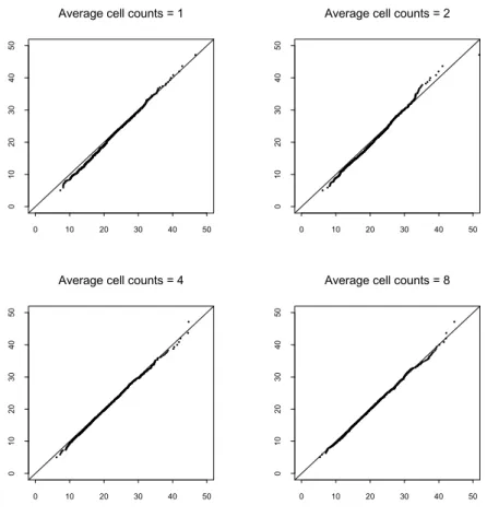
We first provide a small simulation study to check accuracy in finite samples of the limiting distribution of our chi-squared test statistic. We have tried many configurations but almost all of them show almost the same results unless the number d ^p of cells is small. Therefore we present the results for the case where p = 3 , d = 3 so that the limiting distribution of the chi-square statistic is the chi-squared distribution with 20 degrees of freedom.

We consider four different sample sizes, n = 27,54,96 and 196, which have an average of 1, 2, 4 and 8 observations per cell, respectively.

For each sample size n , we generate 500 samples of size n from N ₃ (0, I )

and then calculate the chi-squared statistics for each of them. These 500 values are plotted against the corresponding quantiles of the limiting chi-squared

distribution. The resulting chi-squared probability plots are displayed in Figure 1.

Each plot displays the reference line with slope 1 and intercept 0, which corresponds to the ideal case where empirical and theoretical distributions coincide.

Examining the plots, we see that the limiting distribution is an excellent approximation for the cases where average cell counts is 4 and 8 and that it is reasonably good for the cases where average cell counts is 1 and 2.

We next provide an illustrative example of application to geyser data. There are two time series in geyser data and the waiting time between eruptions is used for our example (see Azzalani and Bowman (1990) for details). We compare the power of our method with those of three popular tests for multivariate normality. The skewness and kurtosis tests of Mardia (1970) and the Q _n test (with Cholesky implementation) of Ozturk and Romeu (1992) have been selected for comparison

Figure 1. Chi-Squared Probability Plots

•••••••••••••••••••••••••••••••••••••••••••••••••••••••••••••••••••••••••••••••••••••••••••••••••••••••••••••••••••••••••••••••••••••••••••••••••••••••••••••••••••••••••••••••••••••••••••••••••••••••••••••••••••••••••••••••••••••••••••••••••••••••••••••••••••••••••••••••••••••••••••••••••••••••••••••••••••••••••••••••••••••••••••••••••••••••••••••••••••••••••••••••••••••••••••••••••••••••••••••••••••••••••••••••••••••••••••••••••••••••••••••••••••••••••••••••••••••••••••••••••••••••••••••••••••••••••••••••••••••••••••••••••••••••••••••••••••••••••••••••••••••••••••••••••••••••••••••••••••••••••••••••••••••••••••••••••••••••••••••••••••••••••••••••••••••••••••••••••••••••••••••••••••••••••••••••••••••••••••••••••••••••••••••••••••••••••••••••••••••••••••••••••••••••••••••••••••••••••••••••••••••••••••••••••••••••••••••••••••••••••••••••••••••••••••••••••••••••••••••••••••••••••••••••••••••••••••••••••••••••••••••••••••••••••••••••••••••••••••••••••••••••••••••••••••••••••••••••••••••••

•

Average cell counts = 1

0 10 20 30 40 50

01020304050

• ••••••••••••••••••••••••••••••••••••••••••••••••••••••••••••••••••••••••••••••••••••••••••••••••••••••••••••••••••••••••••••••••••••••••••••••••••••••••••••••••••••••••••••••••••••••••••••••••••••••••••••••••••••••••••••••••••••••••••••••••••••••••••••••••••••••••••••••••••••••••••••••••••••••••••••••••••••••••••••••••••••••••••••••••••••••••••••••••••••••••••••••••••••••••••••••••••••••••••••••••••••••••••••••••••••••••••••••••••••••••••••••••••••••••••••••••••••••••••••••••••••••••••••••••••••••••••••••••••••••••••••••••••••••••••••••••••••••••••••••••••••••••••••••••••••••••••••••••••••••••••••••••••••••••••••••••••••••••••••••••••••••••••••••••••••••••••••••••••••••••••••••••••••••••••••••••••••••••••••••••••••••••••••••••••••••••••••••••••••••••••••••••••••••••••••••••••••••••••••••••••••••••••••••••••••••••••••••••••••••••••••••••••••••••••••••••••••••••••••••••••••••••••••••••••••••••••••••••••••••••••••••••••••••••••••••••••••••••••••••••••••••••••••••••••••••••••••••••••• •••

•

Average cell counts = 2

0 10 20 30 40 50

01020304050

••••••••••••••••••••••••••••••••••••••••••••••••••••••••••••••••••••••••••••••••••••••••••••••••••••••••••••••••••••••••••••••••••••••••••••••••••••••••••••••••••••••••••••••••••••••••••••••••••••••••••••••••••••••••••••••••••••••••••••••••••••••••••••••••••••••••••••••••••••••••••••••••••••••••••••••••••••••••••••••••••••••••••••••••••••••••••••••••••••••••••••••••••••••••••••••••••••••••••••••••••••••••••••••••••••••••••••••••••••••••••••••••••••••••••••••••••••••••••••••••••••••••••••••••••••••••••••••••••••••••••••••••••••••••••••••••••••••••••••••••••••••••••••••••••••••••••••••••••••••••••••••••••••••••••••••••••••••••••••••••••••••••••••••••••••••••••••••••••••••••••••••••••••••••••••••••••••••••••••••••••••••••••••••••••••••••••••••••••••••••••••••••••••••••••••••••••••••••••••••••••••••••••••••••••••••••••••••••••••••••••••••••••••••••••••••••••••••••••••••••••••••••••••••••••••••••••••••••••••••••••••••••••••••••••••••••••••••••••••••••••••••••••••••••••••••••••••••••• ••••••

•

Average cell counts = 4

0 10 20 30 40 50

01020304050

•• •••••••••••••••••••••••••••••••••••••••••••••••••••••••••••••••••••••••••••••••••••••••••••••••••••••••••••••••••••••••••••••••••••••••••••••••••••••••••••••••••••••••••••••••••••••••••••••••••••••••••••••••••••••••••••••••••••••••••••••••••••••••••••••••••••••••••••••••••••••••••••••••••••••••••••••••••••••••••••••••••••••••••••••••••••••••••••••••••••••••••••••••••••••••••••••••••••••••••••••••••••••••••••••••••••••••••••••••••••••••••••••••••••••••••••••••••••••••••••••••••••••••••••••••••••••••••••••••••••••••••••••••••••••••••••••••••••••••••••••••••••••••••••••••••••••••••••••••••••••••••••••••••••••••••••••••••••••••••••••••••••••••••••••••••••••••••••••••••••••••••••••••••••••••••••••••••••••••••••••••••••••••••••••••••••••••••••••••••••••••••••••••••••••••••••••••••••••••••••••••••••••••••••••••••••••••••••••••••••••••••••••••••••••••••••••••••••••••••••••••••••••••••••••••••••••••••••••••••••••••••••••••••••••••••••••••••••••••••••••••••••••••••••••••••••••••••••••••••• •••

•

Average cell counts = 8

0 10 20 30 40 50

01020304050

since they performed quite well in an extensive simulation study of Romeu and Ozturk (1993). We will examine the multivariate structure of the residuals from fitting a time series model to the waiting time.

We use an automatic procedure called AR in S-Plus to select one of the best autoregressive models based on the Akaike information criterion. By using Yule-Walker equations to estimate the autoregression coefficients, the procedure have chosen AR(2) model. Both autocorrelation and partial autocorrelation functions are well inside the error bars up to 25 lags and the value of Shapiro and Wilk (1965) W test statistic is 0.9822 with p-value 0.3654. Therefore we could not find unusual pattern by the usual time series diagnostics and a univariate test of normality.

We now examine the residuals by our method and other competitors for multivariate normality. To obtain multivariate observations, we divide the residuals into subseries of three consecutive residuals and take each subseries as an observation. In this way, we obtain 99 multivariate observations. Our method with d = 3 leads to chi-squared value 34.46 with an (asymptotic) p-value .0232 and d = 4 leads to chi-squared value 78.01 with an (asymptotic) p-value .0179.

Therefore, our method signals there are some multivariate structure in the residuals. However, other competitors could not detect this structure: Marida's skewness and kurtosis have (asymptotic) p-values 0.160 and 0.569, respectively and the test based on Q n has (asymptotic) p-value 0.601. Therefore, in this example, our test has more power than other tests.

References

1. Azzalini, A., and Bowman, A.W. (1990). A Look at Some Data on the Old Faithful Geyser, Applied Statistics, 39, 357-365.

2. Chernoff, H., and Lehmann, E.L. (1954). The Use of Maximum Likelihood Estimates in χ ² Tests for Goodness of Fit, Annals of Mathematical Statistics, 25, 579-586.

3. Farebrother, R.W. (1990). The Distribution of a Quadratic Form in Normal Variables, Applied Statistics, 39, 294-309.

4. Huffer, F.W. and Park, C. (2002). The Limiting Distribution of a Test for Multivariate Structure, Journal of Statistical Planning and Inference, 105, 417-431.

5. Imhof, J.P. (1961). Computing the Distribution of Quadratic Forms in Normal Variables, Biometrika, 48, 419-426.

6. Mardia, K.V. (1970). Measures of Multivariate Skewness and Kurtosis with Applications, Biometrika, 57, 519-530.

7. Nikulin, M.S. (1973). Chi-Square Test for Continuous Distributions with

Shift and Scale Parameters, Theory of Probability and Its Applications, 18, 559-568.

8. Ozturk, A. and Romeu, J.L. (1992). A New Method for Assessing Multivariate Normality with Graphical Applications, Communications in Statistics - Simulations and Computation, 21, 15-34.

9. Rao, C.R., and Mitra, S.K. (1971). Generalized Inverse of Matrices and Its Applications, John Wiley & Sons, New York.

10. Rao, C.R., and Robson, D.S. (1974). A Chi-Square Statistic for

Goodness-of-Fit Tests within the Exponential Family, Communications in Statistics, 3, 1139-1153.

11. Romeu, J.L. and Ozturk, A. (1993). A Comparative Study of Goodness-of-fit Tests for Multivariate Normality. Journal of Multivariate Analysis, 46, 309-34.

12. Shapiro, S.S. and Wilk, M.B. (1965). An Analysis of Variance Test for Normality (Complete Samples), Biometrika, 52, 591-611.

13. Solomon, H., and Stephens, M.A. (1977). Distribution of a Sum of Weighted Chi-Square Variables, Journal of the American Statistical Association, 72, 881-885.

[ received date : Sep. 2003, accepted date : Nov. 2003 ]