Vol. 22, No. 9 pp. 44-55, 2021
Evaluation of Grain Production Efficiency in the Main Grain
Producing Areas in China Based on a Three Stage DEA Model
Shuang-Yu Hu, Shi-Yong Piao, Yu-Cong Sun, Zhi-Run Li, Sung-Chan Kim, Jong-In Lee*
Department of Agricultural & Resource Economics, Kangwon National University
3단계 DEA를 이용한 중국 식량 주요 생산지역의 효율성 분석에
관한 연구
호쌍우, 박세영, 손우총, 이지윤, 김성찬, 이종인*
강원대학교 농업자원경제학과
Abstract There is a great theoretical and practical significance attached to the reasonable evaluation of the efficiency of grain production, recognition of the current situation of grain production, and exploration of effective ways to improve grain production efficiency against the background of the limited cultivable area and rapid progress of urbanization. Based on the data of 13 main grain-producing areas in China from 2007 to 2019, this study adopted the method of three-stage data envelopment analysis (DEA) to analyze agricultural production efficiency. The results revealed that exogenous environmental variables had a marked impact on grain production efficiency. The three-stage DEA model can reflect the level of food production efficiency in the main grain-producing areas more accurately, so the focus should be on formulating efficiency improvement strategies according to the local realities.
요 약 식량 생산 효율성은 경제 및 자원 사회의 지속가능한 발전의 중요한 요인이며, 중국의 식량안보 및 지역 경제의 평가 척도가 된다. 경지면적이 제한되고 도시화가 급속히 진행되는 배경에서 식량 생산 효율성을 합리적으로 평가하고 식량 생산 현황을 정확히 인식하며 식량 생산 효율성을 높이는 효과적인 경로를 모색하는 것은 중요한 이론과 현실적 의미가 있다. 본 연구는 3단계 DEA 모델을 이용하여 2007년부터 2019년까지의 자료를 바탕으로 중국에 있는 식량 주요 생산지역의 생산 효율성을 분석하였다. 외부환경변수인 도시화율, 농업 보조금 및 1인당 순수익이 중국 지역의 생 산 효율성에 많은 영향을 미치고 있는 것으로 분석되었다. 외부환경 및 임의오류를 제외한 후 중국 식량 주요 생산지역 의 생산 효율성은 0.916에서 0.918로 증가하였고, 순수기술 효율성은 0.953에서 0.965로 증가하였으며, 규모 효율성은 0.962에서 0.952로 감소하였다. 분석결과, 중국 식량 주요 생산지역의 각 성은 생산 효율성을 개선하기 위해 각성의 특성에 적합한 생산 특정에 따라 관리수준을 제고하거나 생산규모를 확대해야 하는 것으로 분석되었다.
Keywords : Main Grain Producing Area, Exogenous Environment Variables, Three-Stage DEA, Grain Production Efficiency, Food Security
*Corresponding Author: Jong-In Lee(Kangwon National Univ.) email: [email protected]
Received May 31, 2021 Revised July 13, 2021 Accepted September 3, 2021 Published September 30, 2021
1. Introduction
As an important strategic material, food security issues are related to the national economy and people's livelihood and are an important foundation and guarantee for national security, social stability, and economic development. As a substantial base and core area of grain production in China, the main grain producing areas have an important strategic position in ensuring the safety and effective supply of national grain production[1]. In 2019, the country’s total grain output was 663.84 million tons, of which the 13 main grain producing areas produced 522.71 million tons, accounting for 78.9% of the country’s total grain output. The main grain producing areas are the key to ensuring effective grain supply and realizing food security, which directly affect the country’s stability and development.
However, there have been some fluctuations in the domestic grain market since 2020, highlighting that the foundation of China’s food security still has some weak links. On the one hand, the structural contradictions of China’s grain are prominent. The stocks of rations such as rice and wheat are sufficient, and the supply is relatively loose. There is a gap in production and demand for feed grains such as corn and soybean, and the relationships between supply and demand are tightening. The food security in China is still not optimistic, the dependence on grain supply and import has further increased, and the self-sufficiency ratio (SSR) of grain is low[2,3]. China is a country with a low risk of food production, but under the background of COVID-19, Chinese people are more concerned about food security, and the world’s grain market is more sensitive, many grain exporting countries have successively restricted grain exports, and the global grain supply chain has been significantly affected. On the other hand, under more people and less land, tightening of resource
and environment carrying capacity, and continuous upgrading of residents’ consumption structure, China will maintain a tight balance of total grain production and demand for a long time. At present, the supply of arable land in China has reached its limit, and with the in-depth development of urbanization level, the area of arable land will show a downward trend.
In the long run, it is no longer possible for food production to rely solely on exploiting the land potential and increasing inputs in production factors[4,5]. In this context, it is necessary to realize the growth of grain output, guarantee national food security, transform grain production methods, and promote the increase of grain output from depending on input to depending on the improvement of production efficiency. Therefore, it is of great significance to rationally evaluate the efficiency of food production, recognize the current situation of food production, and explore practical ways to improve food production efficiency.
In recent years, a numbers of scholars have adopted the traditional data envelopment analysis to study the efficiency of China’s grain production efficiency-from input-output perspective. Xiao Hongbo[6] used DEA and Malmquist index to measure the changes in the comprehensive technical efficiency of China’s grain production from 2004 to 2012 and explored the driving forces and challenges of China’s grain production. Ma Linjing[7] used the DEA-Malmquist method to measure the grain production efficiency of the main grain producing areas, main grain consuming areas from 2001 to 2010 based on the grain production panel data of 31 provinces in China, and analyzed their technical efficiency from the perspective of temporal and spatial differences.
Xue Long[8] analyzed the current situation and adjustment direction of grain production efficiency by DEA-Tobit in Henan Province, used the urban areas from 2000 to 2010 as the
Fig. 1. Map of main grain producing areas in China research unit. To sum up, using DEA to measure grain production efficiency has been more research results in academia, but the single method of using DEA model ignores the impact of environmental factors and may cause overestimation or underestimation of efficiency[9]. This study employed a three-stage DEA model, which was proposed by Fried[10], to incorporate environmental effects and statistical noise into efficiency evaluation. A sample set of 13 provinces of main grain producing areas in China from 2007 to 2019 were analyzed to calculate the efficiency of grain production in China throught the study period.
2. Main grain producing areas overview
Main grain producing areas are mainly referred to the geographical climate conditions such as soil is suitable for food crops, and have a particular resource advantage in technical advantages and economic benefits to satisfy local food consumption based on key products can
provide a large number of commodity grain output, including Heilongjiang, Liaoning, Inner Mongolia, Jilin, Hebei, Henan, Shandong, Jiangsu, Anhui, Jiangxi, Hubei, Hunan, Sichuan, and other 13 provinces, as shown in Fig. 1.
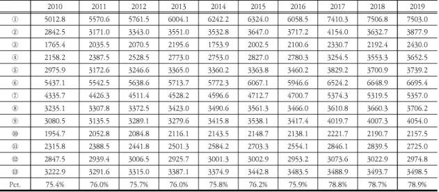
In this study, according to the interpretation of the main statistical indicators of the National Bureau of Statistics of China, grain is classified according to crop varieties, including rice, wheat, corn, tuber corp, and legume corp. As shown in Table 1, in 2019, the country’s total grain output was 663.84 million tons, of which the 13 main grain production areas produced 522.71 million tons, accounting for 78.9% of the country’s total grain output.
3. Methodology
The three-stage DEA model is a method proposed by Fried et al. (2002), which can better evaluate the efficiency of Decision Making Unit (DMU).
(unit: ten thousand tons)
2010 2011 2012 2013 2014 2015 2016 2017 2018 2019
① 5012.8 5570.6 5761.5 6004.1 6242.2 6324.0 6058.5 7410.3 7506.8 7503.0
② 2842.5 3171.0 3343.0 3551.0 3532.8 3647.0 3717.2 4154.0 3632.7 3877.9
③ 1765.4 2035.5 2070.5 2195.6 1753.9 2002.5 2100.6 2330.7 2192.4 2430.0
④ 2158.2 2387.5 2528.5 2773.0 2753.0 2827.0 2780.3 3254.5 3553.3 3652.5
⑤ 2975.9 3172.6 3246.6 3365.0 3360.2 3363.8 3460.2 3829.2 3700.9 3739.2
⑥ 5437.1 5542.5 5638.6 5713.7 5772.3 6067.1 5946.6 6524.2 6648.9 6695.4
⑦ 4335.7 4426.3 4511.4 4528.2 4596.6 4712.7 4700.7 5374.3 5319.5 5357.0
⑧ 3235.1 3307.8 3372.5 3423.0 3490.6 3561.3 3466.0 3610.8 3660.3 3706.2
⑨ 3080.5 3135.5 3289.1 3279.6 3415.8 3538.1 3417.4 4019.7 4007.3 4054.0
⑩ 1954.7 2052.8 2084.8 2116.1 2143.5 2148.7 2138.1 2221.7 2190.7 2157.5
⑪ 2315.8 2388.5 2441.8 2501.3 2584.2 2703.3 2554.1 2846.1 2839.5 2725.0
⑫ 2847.5 2939.4 3006.5 2925.7 3001.3 3002.9 2953.2 3073.6 3022.9 2974.8
⑬ 3222.9 3291.6 3315.0 3387.1 3374.9 3442.8 3483.5 3488.9 3493.7 3498.5
Pct. 75.4% 76.0% 75.7% 76.0% 75.8% 76.2% 75.9% 78.8% 78.7% 78.9%
Source: China Statistical Yearbook 2009-2020
Table 1. Grain output in main grain producing areas 2007-2019
3.1 Stage 1: Traditional DEA model
In the first stage, we apply DEA to input and output data to obtain an initial evaluation of producer performance. This evaluation does not account for the impacts of either the operating environment or statistical noise on producer performance.
The traditional DEA model is proposed by Charnes, Cooper and Rhodes (CCR model)[11].
Banker, Charnes, and Cooper (BCC model)[12]
extended the CCR model and proposed the BCC model under the assumption of Variable Returns to Scale (VRS) in 1984. Technical efficiency (TE) relates to the productivity of inputs. The technical efficiency of a firm is a comparative measure of how well it actually processes inputs to achieve its outputs, as compared to its maximum potential for doing so, as represented by its production possibility frontier (TE=1). A firm is said to be technically inefficient (0<TE<1) if it operates below the frontier.
The BCC model splits the technical efficiency resulting from the CCR model into two parts:
pure technical efficiency (PTE), which overlooks the influence of scale size by only comparing a
DMU to unit of similar scale and measures how a DMU utilizes its sources under exogenous environment. And scale efficiency (SE), which measures how the scale size effects efficiency. If after applying both constant return to scale (CRS), variable returns to scale (VRS) model on the same data, there is an alteration in the two technical efficiencies, this designates that DMU has a scale efficiency and can be calculated by:
SE=TE/PTE. SE is not greater than 1, for a BCC-efficient DMU, i.e., in the most productive scale size, its scale efficiency is 1.
Suppose a system has DMUs, input and output vectors, the input and output vectors of the DMU are respectively.
⋯
(1)
⋯
⋯
Under the Variable Returns to Scale (VRS) model, the BCC model introduces the slack variable values and .
min (2)
≥ ≥ ≥
Where demonstrates the technical efficiency value of each DMU, and implies a dimensional weight vector of the DMU. If
, , the DEA of DMU is considered to be effective, if , , are not all 0, then the DEA of DMU is considered to be weakly effective, if , then the DEA of DMU is not effective.
3.2 Stage 2: Similitude analysis for the stochastic
frontier analysis (SFA) model
After the traditional DEA model analysis, the input slacks of all DMUs are influenced by the external environment parameters, managerial inefficiency, and statistical noises. Following Fried[10], we built up stochastic frontier analysis regression formulation.
(3)
⋯ ⋯
Where, represents the slack variable of input item of the DMU, represents observable environmental variables in the amount of P, implies the coefficients of the environmental variables,
represents the effect of environment variable on input slack variable , represents composed error,
represents managerial inefficiency term as
∼,
illustrates the statistical noises as ∼ , and , aredistributed independently. Let , the closer the value of is to 1, the more managerial factors dominate the error part of the model, the closer the value of is to 0, the more statistical noise dominates the error part of the model.
According to the results of SFA model, the input vectors of the DMUs are adjusted to increase the input for the DMUs with better external environment.
max
max
(4)
⋯ ⋯
where is the input before adjustment,
implies the input after adjustment, are the coefficients of the environment variables,
illustrates the statistical noise. In Eq. (4),
max
represents to adjust all DMUs to the same external environment.
max
represents to adjust all statistical noise of DMUs to the same situation.3.3 Stage 3: The adjusted DEA model
This phase improved measures of managerial efficiency, the adjustment data obtained in the second stage was replaced by the original actual value , then repeated the first stage analysis by applying DEA to the adjusted data.4. Indicator selection and data source
4.1 Input and output indicators
Selecting appropriate indicators is crucial for achieving a comprehensive and objective evaluation of the efficiency of grain production.
Item Planting area Fertilizer usage Irrigated area Machinery usage Labor input Grain output 0.974***
(0.000) 0.899***
(0.000) 0.941***
(0.000) 0.853***
(0.000) 0.715***
(0.000) Note: *** Correlation is significant at the 0.01 level (2-tailed).
Table 3. Pearson correlation test of the input and output indicators.
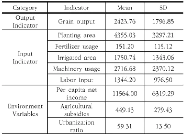
According to the conclusions of literature research and the availability of data[6-8], the input and output indicators are selected as follows, this study selected grain output of main grain producing areas as an output variable, including the output of rice, wheat, corn, tuber corp, and legume corp. According to National Farm Product Cost-benefit Survey, we obtained the input and output information of grain production, so we directly selected the following four indicators as input variables, which mainly includes the plant area, fertilizer usage, the irrigated area, machinery usage, and labor input.
According to the agricultural conditions and a large number of literature references, the input and output variables are selected to measure by three-stage model, as shown in Table 2.
Category Indicator Mean SD
Output
Indicator Grain output 2423.76 1796.85
Input Indicator
Planting area 4355.03 3297.21 Fertilizer usage 151.20 115.12
Irrigated area 1750.74 1343.06 Machinery usage 2716.68 2370.12 Labor input 1344.20 976.50
Environment Variables
Per capita net
income 11564.00 6319.29
Agricultural
subsidies 449.13 279.43
Urbanization
ratio 59.31 13.50
Table 2. Input and output indicators and environment variables
The DEA models requires that the input and output variables are positively correlated-that is, an increase in the input variables cannot cause a decrease in the out variables[13,14]. This paper adopts the Pearson correlation to test the
correlation between inputs and outputs, as shown in Table 3, the selected input and output variables are consistent with the requirements of DEA.
4.2 Environment variables
Environmental variables refer to the factors that can affect grain production efficiency but are not within the subjective control of agriculture. Due to environmental factors, the efficiency of those individuals in a better environment may be higher, while the efficiency of those individuals in a worse environment may not be ideal. Therefore, environmental variables are introduced in the second stage of the analysis, and the influence of environmental variables on efficiency is eliminated. Referring to the existing literature and considering the actual situation and data availability, the following indicators are mainly selected, the per capita net income, agricultural subsidies, urbanization ratio, and other aspects taffect agricultural output[9-14]. These external factors will have a certain impact on agricultural production efficiency, which is specifically analyzed as follows.
1) Per capita net income: It is generally believed that regions with a stronger economy have more basic conditions that are favorable to the improvement of grain production efficiency[1].
In this study, the per capita net income was employed to characterize regional economic development. Since the per capita net income in grain production cannot be obtained directly from the statistical yearbook, we need to process the data as follows, the per capita net income in grain production, it is calculated by the
prodortion of agricultural income in the total household income[14].
2) Agricultural subsidies: Regarding the related policies of financial support for agriculture, this study considers that the agricultural subsidies can increase farmers’ enthusiasm for farming[9], and the support of subsidy policy is of great significance to grain production. In consideration of the availability of data, this study uses agricultural subsidies to measure the impact of national policies on grain production, which is represented by grain production subsidies in local fiscal expenditures[14].
3) Urbanization ratio: The increase in the urbanization ratio means an increase in the opportunity cost of labor, and the supply of factor resources is tight. Agricultural production must develops in the direction of intensification, which is beneficial to improving of agricultural production efficiency[5]. The urbanization ratio is represented by the proportion of the urban population in the total population.
4.3 Data source
Considering the integrity and availability of data, the data used in this paper is from for the years 2007-2019. Those data collected from China Statistical Yearbook (2008-2020) and National Farm Product Cost-benefit Survey (2008-2020).
5. Empirical study of the efficiency of
China’s main grain producing areas
5.1 The results of the DEA model: Stage 1
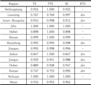
In stage 1, the DEAP 2.1 was used to measure grain production efficiency. Table 4 shows the mean values of efficiency of grain production during the 2007-2019 and the returns to scale in 2019. The mean value for technical efficiency (TE), pure technical efficiency (PTE), and scale
efficiency (SE) for stage 1, was 0.916, 0.953, and 0.962, respectively. pure technical efficiency and scale efficiency were the factors that limited the grain production efficiency in China. In addition, Heilongjiang, Jilin, Heibei, Heinan, Jiangsu, Sichuan were at the frontier of efficiency. Seven provinces and municipalities, such as Inner Mongolia, Anhui, were high in PTE, indicating they had weak DEA efficiency. PTE and SE of the remaining provinces and municipalities could be further improved.
Region TE PTE SE RTS
Heilongjiang 0.933 1.000 0.933 -
Liaoning 0.767 0.769 0.997 drs
Inner Mongolia 0.910 0.998 0.912 drs
Jilin 1.000 1.000 1.000 -
Hebei 0.898 1.000 0.898 -
Henan 0.999 1.000 0.999 -
Shandong 0.992 0.993 0.998 drs
Jiangsu 0.993 0.998 0.996 -
Anhui 0.847 1.000 0.847 drs
Jiangxi 0.929 0.941 0.988 drs
Hubei 0.889 0.938 0.947 drs
Hunan 0.747 0.755 0.990 drs
Sichuan 1.000 1.000 1.000 -
Mean 0.916 0.953 0.962
Note: “TE”, “PTE”, “SE”, and “RTS” represent technical efficiency, pure technical efficiency, scale efficiency, and return to scale, respectively. In addition, “irs”, “drs”, and “-”
signify that the return to scale increased, decreased, or remained unchanged, respectively.
Table 4. Grain production efficiency in 2007-2019:
Stage 1
5.2 The results of the stochastic frontier
analysis model : Stage 2
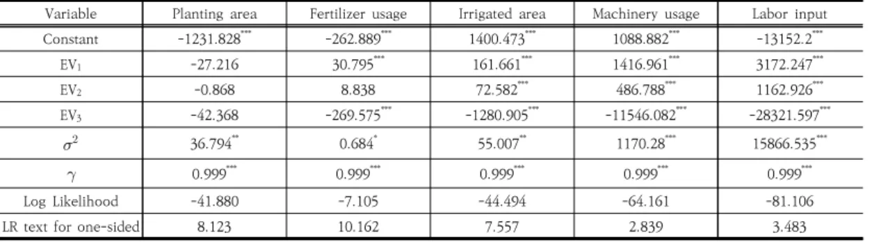
According to Table 5, the Likelihood Ratio (LR) test for one-sided of the SFA model passed the significance test at the 1% level and rejected the null hypothesis that there was no managerial inefficiency, indicating that it was reasonable to apply the SFA model. The slack variables of the input variables in stage 1 are regarded as the dependent variable, and the three environmental variables (Per capita net income, Agricultural
Variable Planting area Fertilizer usage Irrigated area Machinery usage Labor input
Constant -1231.828*** -262.889*** 1400.473*** 1088.882*** -13152.2***
EV1 -27.216 30.795*** 161.661*** 1416.961*** 3172.247***
EV2 -0.868 8.838 72.582*** 486.788*** 1162.926***
EV3 -42.368 -269.575*** -1280.905*** -11546.082*** -28321.597***
36.794** 0.684* 55.007** 1170.28*** 15866.535***
0.999*** 0.999*** 0.999*** 0.999*** 0.999***
Log Likelihood -41.880 -7.105 -44.494 -64.161 -81.106
LR text for one-sided 8.123 10.162 7.557 2.839 3.483
Note: *: p<0.1, **: p<0.05, ***: p<0.01
Table 5. The results (2019) of the SFA model: Stage 2
Technical efficiency Pure technical efficiency Scale efficiency
Stage 1 Stage 2 Stage 1 Stage 2 Stage 1 Stage 2
Grain
output 0.322***
(0.000) 0.624***
(0.000) 0.084***
(0.000) 0.233***
(0.000) 0.082***
(0.000) 0.523***
(0.000) Note: *: p<0.1, **: p<0.05, ***: p<0.01
Table 6. Spearman rank correlation
subsidies, Urbanization ratio) are regarded as the independent variables. To ensure the accuracy of the calculation, a yearly cross-sectional regression technique was adopted. The software application, Frontier 4.1, was utilized to perform the stochastic frontier analysis (SFA). Owing to word count limitations, only the results for 2019 are presented in Table 5. Both and value passed the significance test (=0.999), indicating that compared with random error, managerial inefficiency in the mixed error term has a dominant influence on the slack variable. In addition, the estimated coefficients of the four environmental variables also passed the significance test, indicating that environmental factors have a significant impact on the slack values of the planting area, fertilizer usage, the irrigated area, machinery usage, and the labor input. Therefore, applying the SFA model to separate the environmental variables and statistical noises is reasonable.
1) Per capita net income: per capita net income is positive for the input slack variables (fertilizer usage, the irrigated area, machinery usage, and the labor input), and both can pass
the 10% significance test. That is to say, when the per capita net income increase, the slack in input will increase, which will adversely affect the efficiency of grain production. This is just the opposite of theoretical expectations, reflecting that the grain production is still an extensive mode of high input in China.
2) Agricultural subsidies: The increase of agricultural subsidies only has a negative coefficient for the input slack of planting area, but the t-test result is not significant. The input slack variables of fertilizer usage, irrigated area, machinery usage, labor input are all positive, this shows that agricultural subsidies have not played their due role in the grain production efficiency.
Increasing agricultural subsidies will lead to an increase in input slack, that may be because government agricultural subsidies tend to increase farmers’ income expectations and encourage farmers to expand their planting scale, but blindly expanding the scale and increasing input will result in the inefficient of use of factors of production.
3) Urbanization ratio: It can be seen from the above Table 5 that the regression coefficients of
the urbanization ratio to the slack variable are all negative, indicating that the improvement of the level of urbanization can indeed realize the effective allocation of resources, and the increase in the urbanization ratio in main grain producing areas has a positive effect on grain production efficiency.
5.3 The results of the DEA model: Stage 3
The SFA model in stage 2 eliminated the influence of environment factors and statistical noises on efficiency. The adjusted input value was then introduced into the model to replace the orginal input value at stage 1. the efficiency of grain production (Table 7).In order to demonstrate that the efficiency values measured by DEA in the stage 3 are more objective, and to better explain the grain output in main grain producing areas, this study conducted Spearman’s rank correlation analysis on the efficiency values (stage 1 and stage 3) and agricultural output, and the results are shown in Table 6. After adjusting environmental factors in the second stage, the correlation between TE, PTE, and SE of the main grain producing areas and agricultural output has been significantly improved, which shows that the adjustment of the second stage is necessary. The result of the third stage can reflect the managerial efficiency more truly than the first stage.
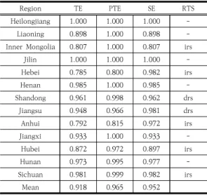
In stage 3, the DEAP 2.1 was used to measure grain production efficiency without considering the impact of external environment variables.
The mean values of efficiency of grain production during the 2007-2019 and the returns to scale in 2019, as shown in Table 7. The mean value for technical efficiency (TE), pure technical efficiency (PTE), and scale efficiency (SE) for stage 3, without considering the impact of external environment variables, was 0.918, 0.965, and 0.952, respectively. After removing the influence of the external environment parameters, managerial inefficiency, and statistical noises, on
the provincial level, Heilongjiang, Liaoning, Jinlin, Heinan, Jiangxi, Hunan were at the frontier of efficiency. The finding confirms that the grain production efficiency of Heilongjiang, Jilin, and Henan remained consistently high, as they remained at the efficient frontier. The efficiency of Liaoning, Hunan significantly changed after the model adjustments, indicating that environmental factors have a considerable impact on these provinces/municipalities. In addition, the TE of Hebei, Inner Mongolia decreased after the model adjustment.
Region TE PTE SE RTS
Heilongjiang 1.000 1.000 1.000 -
Liaoning 0.898 1.000 0.898 -
Inner Mongolia 0.807 1.000 0.807 irs
Jilin 1.000 1.000 1.000 -
Hebei 0.785 0.800 0.982 irs
Henan 0.985 1.000 0.985 -
Shandong 0.961 0.998 0.962 drs
Jiangsu 0.948 0.966 0.981 drs
Anhui 0.792 0.815 0.972 irs
Jiangxi 0.933 1.000 0.933 -
Hubei 0.872 0.972 0.897 irs
Hunan 0.973 0.995 0.977 -
Sichuan 0.981 0.999 0.982 irs
Mean 0.918 0.965 0.952
Note: “TE”, “PTE”, “SE”, and “RTS” represent technical efficiency, pure technical efficiency, scale efficiency, and return to scale, respectively. In addition, “irs”, “drs”, and “-”
signify that the return to scale increased, decreased, or remained unchanged, respectively.
Table 7. Grain production efficiency in 2007-2019:
Stage 3
6. Conclusions and suggestions
This study employed a three-stage DEA model to analyze the efficiency of main grain producing areas in China from 2007 to 2019. The conclusions are follows. (1) Before and after stage 2 of adjustment, the grain production efficiency of provinces and municipalities has changed, indicating that environmental variables
and random errors have significantly impacted grain production efficiency. This study conducted Spearman’s rank correlation analysis on the efficiency values (stage 1 and stage 3) and agricultural output. The results indicate the application of the three-stage DEA model is more reasonable and accurate than the traditional DEA method to measure agricultural production efficiency. (2) Through the second stage of SFA regression analysis, it is found that environmental variables have significant effects on agricultural production efficiency. Among the environmental variables, rural households’ per capita net income is the unfavorable factor of agricultural production. The improvement of the urbanization level can realize the effective allocation of resources to improve agricultural production efficiency. Agricultural subsidies have no due effect on agricultural production efficiency. Increasing agricultural subsidies will lead to an increase in input slack. (3) After removing environmental variables and random errors, the national average technical efficiency increased from 0.916 to 0.918. The average pure technical efficiency increased from 0.953 to 0.965, and the average scale efficiency decreased from 0.962 to 0.952. The agricultural scale state of most provinces and cities also changed from the decreasing return to scale to the increasing return to scale.
The above conclusions give us two main enlightenment as follows. First, because the environmental variables and random errors significantly impact agricultural production efficiency, random errors are uncontrollable factors, so the control of environmental variables is one of the inevitable choices to improve agricultural production efficiency. According to the analysis of three environmental variables, the first thing we should do is continue the orderly urbanization level, and give full play to the promotion of urbanization force on agricultural production efficiency. In addition, the farmers’
income and agricultural subsidies have a negative impact on agricultural production efficiency that does not mean to reduce the farmers’ income and agricultural subsidies, increasing farmers’ income is one of the themes of the “three rural” construction, on the premise of guarantee the farmers’ income, to change or weaken the current farmers’ income level to the negative impact of agricultural production efficiency, we should strengthen the guide of farmers, and expand its effective investment channels so that it can realize the effective allocation of income rather than blind investment. As for agricultural subsidies, the overall level of agricultural subsidies in China is not high, and agricultural subsidies do not promote agricultural production efficiency as expected but lead to the waste of agricultural production input. Therefore, the project portfolio of agricultural subsidies should be improved to promote agricultural production efficiency. Secondly, the characteristics of agricultural production efficiency of provinces and cities in China’s main grain producing areas are not consistent, so each region should carry out reform according to its own insufficiency of efficiency, rather than blindly follow a certain established mode to develop agriculture.
References
[1] J. H. Guo, M. Ni, B. Y. Li, “Research on Agricultural Production Efficiency Based on Three-Stage DEA model”, The Journal of Quantitative & Technical Economics, Vol.12, No.02, pp.27-38, 2010.
[2] P. M. He, D. S. Li, “An Empirical Study of Grain Yield and Price Fluctuation Based on Food Security”, Journal of Agrotechnical Economics, No.02, pp.85-92, 2009.
[3] Y. Q. Guo, L. Q. Hou, “Study of Measurement and Influencing Factors of Green Total Factor Productivity of Grain Agriculture in Main Grain Producing Areas of China”, Science and Technology Management Research, No.19, pp.224-229, 2020.
[4] J. Tang, J. Vila, “Study on Technical Efficiency and
Influence Factors of Grain Production: panel data from 31 provinces in China from 1990-2013”, Journal of Agrotechnical Economics, no.09, pp.72-83, 2016.
[5] Q. N. Zhang, F. F. Zhang, X. J. Chen, “Research on Calculation of Production Efficiency in Main Grain Production Areas in China”, Price: Theory & Practice, No.09, pp.155-158, 2018.
[6] H. B. Xiao, J. M. Wang, “Analysis of China's Grain Technical Efficiency and Total Factor Productivity Since the New Century”, Journal of Agrotechnical Economics, No.01, pp.36-46, 2012.
[7] L. J. Ma, Y. P. Wang, J. Wu, “Spatial Disequilibrium and Convergence Analysis of Technical Efficiency of Grain Production in China”, Journal of Agrotechnical Economics, No.05, pp.4-12, 2015.
[8] L. Xue, Q. Liu, “Analysis of Food Production Technical Efficiency and Total Factor Productivity of Henan Province”, Journal of Henan Agricultural University, Vol.43, No.03, pp.345-350, 2013.
[9] W. W. Chen, “Research on Three-stage DEA model”, Systems Engineering, Vol.32, No.9, pp.144-149, 2014.
[10] H. O. Fried, C. A. K. Lovell, S. S. Schmidt, S.
Yaisawarng, “Accounting for Environmental Effects and Statistical Noise in Data Envelopment Analysis”, Journal of Productivity Analysis, Vol.17, No.1, pp.157-174, 2002.
DOI: https://doi.org/10.1023/A:1013548723393 [11] A. Charnes A, W. W. Cooper, E. Rhodes, “Measuring
the Efficiency of Decision Making Units”, European Journal of Operation Research, Vol.2, No.6, pp.429-444, 1978.
DOI: https://doi.org/10.1016/0377-2217(78)90138-8 [12] Banker, Charne, Cooper, “Some Models for estimating
Technical and Scale Inefficiencies in Data Development Analysis”, Management Science, Vol.30, No.9, pp.1078-1092, 1984.
DOI: https://doi.org/10.1287/mnsc.30.9.1078 [13] Y. M. Hu, Y. J. Wu, W. Zhou, T. Li, L. Q. Li, “A
three-stage DEA-based efficiency evaluation of social security expenditure in China”, PLoS One, Vol.15, No.2, pp.1-12, 2020.
DOI: https://doi.org/10.1371/journal.pone.0226046 [14] Q. Y. Lu, X. H. Meng, “Research on the Agricultural
Production Efficiency of Jiangsu Province Based on the Three-stage Data Envelopment Analysis (DEA) Model”, Journal of Northeast Agricultural Sciences, Vol.46, No.01, pp.94-99, 2021.
Yu-Shuang Hu [Regular member]
• Jun. 2017 : Yanbian Univ., Agriculture and Forestry Economic Management, BM
• Jun. 2019 : Yanbian Univ., Rural Regional Development, MSC(Agr)
• Sept. 2019 ~ current : Kangwon Univ., Dept. of Agricultural and Resource Economics, PhD Program
<Research Interests>
Agriculture Circulation, Consumer Behavior
Shi-Yong Piao [Regular member]
• Jun. 2015 : Yanbian Univ., Agriculture and Forestry Economic Management, BM
• Jun. 2018 : Kangwon Univ., Agricultural and Resource Economics, MSAE
• Sept. 2018 ~ current : Kangwon Univ., Dept. of Agricultural and Resource Economics, PhD Program
<Research Interests>
Livestock Economy, Food Consumption
Yu-Cong Sun [Regular member]
• Jun. 2012 : JiLin Agricultural Univ., Information and Computing Science, BS
• Jun. 2018 : JiLin Univ., Agriculture and Forestry Economic Management, MM
• Sept. 2018 ~ current : Kangwon Univ., Dept. of Agricultural and Resource Economics, PhD Program
<Research Interests>
Livestock Economy, Consumer Behavior
Zhi-run Li [Regular member]
• Jun. 2014 : Jilin Univ., Agriculture and Forestry Economic Management, BM
• Jun. 2019 : Jilin Univ., Rural Regional Development, MSC(Agr)
• Sept. 2019 ~ current : Kangwon Univ., Dept. of Agricultural and Resource Economics, PhD Program
<Research Interests>
Green Agriculture, Sustainable Agriculture
Sung-Chan Kim [Associate member]
• Feb. 2021 : Kangwon Univ., Agricultural and Resource Economics, BSAE
• Mar. 2021 ~ current : Kangwon Univ., Dept. of Agricultural and Resource Economics, MSAE Program
<Research Interests>
Livestock Economy, Food Consumption
Jong-In Lee [Regular member]
• Feb. 1987 : Kangwon Univ., Animal Science, BSC(Agr)
• Feb. 1993 : Kangwon Univ., Livestock Management, MM
• Aug. 1997 : Missouri Univ., Agricultural Economics, MSAE
• Dec. 2000 : Oklahoma Univ., Agricultural Economics, PhD
• Feb. 2006 ~ current : Kangwon Univ., Dept. of Agricultural and Resource Economics, Professor
<Research Interests>
Livestock Management, Livestock Economy, Food Consumption