Fault Tolerant Control of Wind Turbine with Sensor and Actuator Faults

1. INTRODUCTION

In the last decade, wind energy has become an important role among the renewable resources as a reliable and abundant energy source. Recently, as shown in Fig. 1, wind turbines have become larger and more complex with high power outputs [1]. For instance, the capacity of installed wind turbines has increased by 31.69% over the last 10 years [2]. However, their failure rate has correspondingly increased with the number and size of wind turbines.

Further, wind turbines are being increasingly located in remote locations that are offshore, making it difficult to maintain and repair faults. For these reasons, Fault- Tolerant Control (FTC) systems are especially important for the maintenance of wind turbines.

This paper proposes a method for the fault detection, isolation and FTC of the sensors and blade actuators based on a robust dynamic inversion observer and control allocation. By using FTC, many faults in wind turbines can

be reduced, maintaining stability and preventing loss of power efficiency [3, 4]. On the other hand, a robust dynamic inversion observer is adopted in order to tolerate faults in the speed sensors of rotors and generators by accurately tracking measured values [5]. In the case of actuator faults, the control allocation based method is applied in order to tolerate faults in the blade actuator system. Control allocation has been widely used in various control systems, especially in over-actuated systems [6].

The key idea of control allocation is to distribute a desired moment from the control law into several actuators to generate a required output. Each blade can be given a different angle using control allocation when the three blades of the wind turbine are controlled individually. If there are faults in the pitch system, the lost torque due to the faulty blade actuator is redistributed into normal blade actuators according to the reconfiguration law based on control allocation.

In this work, the efficiency of the proposed method is evaluated through computer simulations using a benchmark test model of a wind turbine by considering faults in pitch actuators and speed sensors.

2. WIND TURBINE SYSTEMS

School of Electronics Engineering, Kyungpook National University +Corresponding author: [email protected]

(Received : Dec. 12, 2012, Accepted : Jan. 15, 2013)

This is an Open Access article distributed under the terms of the Creative Commons Attribution Non-Commercial License(http://creativecommons.org/licenses/by- nc/3.0)which permits unrestricted non-commercial use, distribution, and reproduction in any medium, provided the original work is properly cited.

http://dx.doi.org/10.5369/JSST.2013.22.1.28 pISSN 1225-5475/eISSN 2093-7563

Fault Tolerant Control of Wind Turbine with Sensor and Actuator Faults

Jiyeon Kim, Inseok Yang, and Dongik Lee⁺

Abstract

This paper presents a fault-tolerant control technique for wind turbine systems with sensor and actuator faults. The control objective is to maximize power production and minimize turbine loads by calculating a desired pitch angle within their limits. Any fault with a sensor and actuator can cause significant error in the pitch position of the corresponding blade. This problem may result in insufficient torque such that the power reference cannot be achieved. In this paper, a fault-tolerant control technique using a robust dynamic inversion observer and control allocation is employed to achieve successful pitch control despite these faults in the sensor and actuator. The observer based detection method is used to detect and isolate sensor faults by checking whether errors are larger than threshold values. In addition, the control allocation technique is adopted to tolerate actuator fault. Control allocation is one of the most commonly used fault- tolerant control techniques, especially for over-actuated systems. Further, the control allocation method can be used to achieve the power reference even in the event of blade actuator fault by redistributing the lost torque due to erroneous pitch position into non-faulty blade actuators. The effectiveness of the proposed method is demonstrated through simulations with a benchmark model of the wind turbine.

Keywords : Wind turbine, Sensor fault, Actuator fault, Fault detection and isolation, Fault-tolerant control

2.1 Standard regions of control

A typical wind turbine has three operating regions that depend on wind speed as shown in Fig. 2 [7]. The available power in the wind passing through the swept area of the blades can be presented as

where p is the air density, which is assumed to be constant, A is the rotor swept area, and v_wis the wind speed.

As shown by the dashed line in Fig. 2, an ideal wind turbine has a maximum power coefficient of 0.593, which is called the Betz limit [8]. However, there are three main regions of operation as indicated by the solid line, as the actual turbines must limit the captured wind power for safe operation. Region 1 is the wind turbine start-up routine.

Here, the wind speed is too slow such that the turbine does not operate. Region 2 is an operating mode to maximize

power and control the blade actuator system. In Region 3, the turbine power should be maintained at maximum peak power so as not to exceed safe electrical and mechanical loads.

2.2 Wind turbine model structure

Fig. 3 demonstrates the relationship between sub- systems of the wind turbine system: the blade and pitch system, drive train, generator and converter, and controller [9]. The wind speed v_wis input into the wind turbine and the generator power P_g is the system output. The controllable inputs are the pitch angle reference β_r, and the generator torque reference

τ

g,r. P_r denotes the power reference to the controller.

The pitch angle measurement, rotor speed measurement, generator speed measurement, and generator torque measurement are defined as β_m,

ω

r,_m,

ω

g,m, and

τ

g,m, respectively.

2.3 Aerodynamic and Pitch System Model

The output of the aerodynamic model is the aerodynamic torque

τ

r,which is affected by the pitch angle, the speed of the rotor, and the wind speed. The aerodynamic torque applied to the rotor can be expressed as

where R is the radius of the rotor, λ(t) is the tip-speed ratio, and β(t) is the pitch angle. C_qis the rotor torque coefficient table which is derived from the power coefficient by dividing the tip-speed ratio.

When the three blades are controlled individually, total aerodynamic torque is computed by averaging the torque

Fig. 2. Typical power curve for the wind turbine system [7].

Fig. 1. Size evolution of the wind turbine [1].

(1)

Fig. 3. Structure of the wind turbine [9].

(2)

provided by each blade as follows:

The hydraulic pitch actuator system is modelled by a second order system [10].

2.4 Drive train model

The dynamics of the drive train model are given as [9].

where J_rand J_gare the moments of inertia of the low speed shaft and the high speed shaft, respectively. K_dtis the torsion stiffness of the drive train, and B_dtis the torsion damping coefficient of the drive train. B_gis the viscous friction of the high speed shaft, N_gis the gear ratio, η_dtis the efficiency of the drive train, and θ (t) is the torsion angle of the drive train.

2.5 Power system model

The dynamics of the converter is modeled as

The power produced by the generator is given by

where η_g is the efficiency of the generator.

3. SENSOR FAULT DETECTION AND ISOLATION USING ROBUST DYNAMIC INVERSION OBSERVER 3.1 Types of Sensor Faults

Typical sensor faults can be categorized into five types as shown in Fig. 4: bias, drift, loss of accuracy, freezing, and calibration error [11]. If bias fault occurs, then the measured signal has a constant error in comparison with the actual signal. If the error between actual and measured signals increases over time, then fault is categorized as drift sensor fault. If loss of accuracy fault occurs in a sensor, then the sensor cannot measure the true value. In the case of freezing sensor fault, the sensor reports a constant value.

Finally, calibration error cannot accurately represent the actual physical meaning of the relationship between input and output signals of the system.

3.2 The Robust Dynamic Inversion Observer

In this section, the robust dynamic inversion (RDI) observer proposed by Yang et al is introduced [5].

Consider the following linearized system:

Fig. 4. Types of sensor faults [11].

(4)

(8) (3)

where

(5)

(6)

(7)

(9)

where x∈Rⁿand u∈R^mare a state matrix and an input distribution matrix, respectively. Further, ∆A∈R^n-nand ∆B

∈R^n-mare matrices of model mismatches, and d(t)∈Rⁿ is a disturbance vector. Let ξ(t, x(t), u(t)) = ∆Ax(t) + ∆Bu(t) + d(t) with ||ξ(t, x(t), u(t))||² < p, for some positive p. It is assumed that there exists a constant feedback gain matrix G such that A-GC has some stable eigenvalues. Then the RDI observer can be designed as follows:

where v(t) is the discontinuous vector. It is worth noting that an observer is generally used to estimate unmeasured states. However, since sensor faults can be detected by comparing measured values with estimated values, an observer estimates full states, including measured states, using sensors.

Assuming that e(t) = x(t) - x(t), the error dynamics can be represented as:

where A = A-GC. Also, the discontinuous vector term v(t) can be designed using the robust dynamic inversion control method [5] as:

where v_DI(t) = -Ae(t) and v_sw(t) = -Ksgn(e(t)) for some diagonal matrix K with positive diagonal entries k_i(i = 1, 2,

…, n) satisfying p < min(k₁, k₂, …, k_n). Diagonal entries k_i generate boundaries for obtaining robustness of the observer. By substituting (13) into (12), the error dynamics can be represented as follows:

3.3 The Proposed Sensor Fault Detection and Isolation Method

In this section, the fault detection and isolation (FDI) method based on the RDI observer is proposed.

If the system has a sensor fault, then its dynamics can be represented as follows:

where f_s(t, x(t)) is a bounded unknown term due to sensor faults. Let ξ(t, x(t), u(t)) = ∆Ax(t) + ∆Bu(t) + d(t) for the model mismatches ∆A and ∆B and a disturbance d(t) satisfying ||ξ(t, x(t), u(t))||² < p, for some positive p. Then, the RDI observer for sensor FDI can be designed as follows:

where v(t) is the switching term designed as (13).

Let e(t) = y(t) - y(t). Then, the error dynamics can be represented as:

Since the switching input is designed to generate boundaries for robustness, the entries of K are too small to disturb observer performance. Hence, the error dynamics represented in (17) can be reduced as follows:

In (18), if sensor fault occurs, then the error dynamics cannot be converged to zero.

Generally, sensor faults can be detected by checking whether or not errors between measured values and observed values are larger than the user-defined specific qualitative values called threshold values, i.e. for i = 1, 2,

…, n

where the subscript i indicates the i-th sensor and μ_iis the threshold value for the i-th sensor.

Consequently, a sensor fault can be detected and isolated fault occurs in the i-th sensor,

the i-th sensor is healthy (10)

(18) (13)

(11)

⌒

⌒

(12)

(14)

(19) (15)

(17) (16)

⌒

⌒

by checking the errors of measured values and observed values.

4. ACTUATOR FAULT-TOLERANT CONTROL USING CONTROL ALLOCATION

4.1 Control allocation method

Control allocation involves distribution of the redundant controls into several actuators in order to generate a desired moment, which is calculated by the control law. Consider the following continuous system:

where x∈Rⁿis the state vector and u∈R^mis the control input. A∈R^n-n is the state matrix and B_u∈R^n-m is the control effectiveness matrix with rank k < m.

Given a desired moment v∈Rⁿ, the control allocation problem is to determine the optimal actuator input u(t) such that the following is satisfied:

where u_minand u_maxare the lower and upper limits of the actuators, respectively. In other words, given the desired input v(t), the optimal actuator input u(t) that satisfies the equation (21) is determined.

For the wind turbine system with three blades, the equation (21) can be represented as

where

τ

vis the desired aerodynamic torque by the control law and

τ

uis the actual aerodynamic torque input by the control allocation problem.

4.2 The proposed fault-tolerant control method

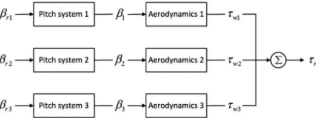
If all blade actuators operate normally, then each blades pitch angle is almost the same. However, if the pitch system in the blade actuator develops a fault, then the aerodynamic torque

τ

rcan be affected by the output of the faulty blade actuator as shown in Fig. 5. If the fault occurs in the blade actuator system, then the control allocation

problem (22) can be represented as

where B_ris the matrix that consists of vector b_r, and

τ

v, f

is the actual aerodynamic torque vector.

τ

ⁿiand

τ

^fi are the actual rotor torques in the normal and faulty blade actuators, respectively. f_iis the condition data transmitted from the Fault Detection and Isolation (FDI) system satisfying,

Then, the reconfiguration law can be represented as follows:

where

τ

^v,ris the composed aerodynamic torque vector, which is composed of

τ

^v,ri for i = 1, 2, 3. The compensated torque in the i-th blade actuator

τ

^v,ri can be written as follows:

where

τ

^reconfi is the additional torque for compensation of the torque lost due to the faulty blade actuator.

τ

^corr is the corrective torque in the normal blade actuator consisting of

τ

ⁿiand

τ

^reconfi. The corrective torque is calculated by the pseudo-inverse method [12].

where β^corr_jis the corrective pitch angle in the j-th normal actuator. In other words, given the tip-speed ratio λ_jand the (20)

normal blade

fauity blade ⁽²⁴⁾

(26)

(27) (21)

(22)

(25) (23)

Fig. 5. Block diagram of pitch systems and aerodynamics.

wind speed

v

_wj, the optimal pitch angle β^corr_jthat satisfies (27) for a set time is determined.

The corrective torque coefficient table Cq,corrj, which includes β^corr_j, can be written as

Initially, the torque coefficient table Cq,tab, satisfying the tip-speed ratio of the j-th actuator λ_j, can be calculated for all of the pitch angles in the coefficient table. Cq-table data are provided by the benchmark model from kk-electronic a/s [9]. The corrective pitch angle βcorrjthat satisfies Cq,corrj, for all values in Cq,tabcan be calculated by using linear interpolation.

5. SIMULATION 5.1 Simulation scenario

In this paper, faults in the drive train sensor and blade actuator were considered in order to evaluate the performances of the proposed fault detection, isolation, and reconfiguration abilities.

The proposed method is evaluated according to a series of computer simulations using a non-linear test benchmark model of a wind turbine provided by kk-electronic a/s, which supplies the electronic system for wind farms [9].

This model is based on a realistic and generic three blades horizontal variable speed wind turbine with a rated power output of 4.8 MW. The wind turbine includes a number of sensors to measure the pitch positions of the three blades, generator speed, and rotor speed. Each part uses two sensors in order to ensure physical redundancy.

Fig. 6 shows the wind speed sequence used in this benchmark model simulation [9]. The real measured wind data from a wind park is shown in Fig. 6(a). This wind speed is used as the input of a wind model during a time period from 4400s. Fig. 6(b) presents the output of the wind model which is the three blade effective wind speed;

that is, wind speeds averaged over the area of the blades.

The controller in this test benchmark model operates in Region 2 and Region 3 as mentioned in Section 2.1. The controller mode is divided into two modes as follows:

Control mode 1: This mode denotes power maximization

and optimization. The generator torque reference and pitch angle reference are given by

where C_pmax is the maximal value of the power coefficient table C_p.

Control mode 2: In this mode, the pitch angle reference is controlled by a PI controller in order to follow the power reference P_r. The generator torque reference is used to limit fast disturbances.

As a sensor fault, a bias fault of 0.5 rad is assumed to be injected into the drive train during the time period from 3,200-3,450s; that is, the torsion angle sensor of the drive train continuously measures the angle with a constant error of 0.5 rad. Thus, f_s(t, x(t)) = [0, 0, 0.5], in (15). It is assumed that random bounded disturbances are injected into this simulation.

The pitch actuator fault scenario used in this work focuses on a changed pitch system response in the third blade actuator due to a fault; that is, the blade actuator parameters,

ω

_n= 11.11 and ζ= 0.6 abruptly change to

ω

_n3= (28)

Fig. 6. Wind speed sequence used in the test model [9].

(a) Real measured wind speed

(b) Effective wind speed

(32)

(33) (34) (29)

(30) (31)

3.42 and ζ₃= 0.9, respectively, during the time period from 3,000-3,500s.

5.2 Simulation results

Figs. 7-8 show the performance of the proposed RDI observer in a fault-free case. As shown in Fig. 8, the errors between measured and observed values are almost zero.

Hence, the observer can accurately track the actual values.

It is worth noting that a chattering problem around the measured value occurs while observing the actual value due to switching the input term v_sw(t) represented in (13) (Fig. 8). However, the chattering problem can be com- pensated for by replacing the sgn function by a continuous function such as a saturation function, etc.

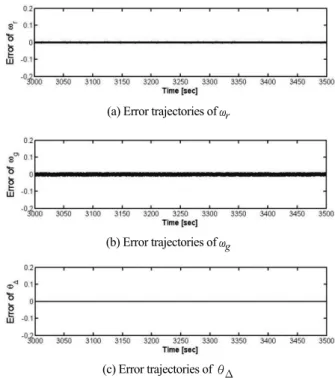
Simulation results for the detection and isolation of a sensor fault in the drive train are described in Figs. 9-11.

During the time period from 3,200-3,450 s, the observer for θ cannot track the actual value with 0.75 rad error as shown in Figs. 9-10. However, values measured by a normal sensor can be accurately tracked by the proposed observer. Hence, the sensor can be detected and isolated.

Fig. 11 presents the outputs of the fault indicator that reports binary values: 0 for the normal case and 1 for the faulty case. In Fig. 11(c), the fault indicator for θ reports 1 during the time period from 3,200-3,450 s while other indicators report 0.

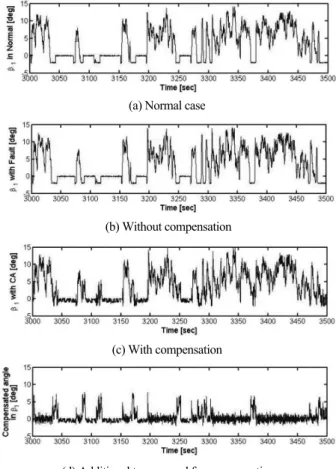
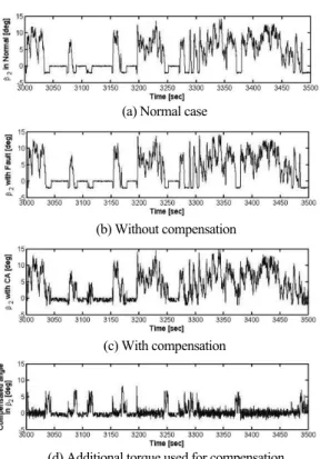
Figs. 12-14 show the pitch angle of each blade for the actuator fault. As shown in Figs. 12 and 13, blade actuators 1 and 2 compensate for the lost pitch angle due to faulty blade actuator 3 by applying an additional pitch angle, which corresponds to the corrective torque. As shown in Figs. 12(d), 13(d), and 14(d), the corrective angle for the third blade, which has a faulty actuator, is almost zero, whereas the corrective angles for the two non-faulty blades are calculated according to the corrective torque.

In Fig. 15, errors in the power generated from the desired power reference in the case of fault are compared; that is, Fig. 15(a) without compensation and Fig. 15(b) with compensation using the proposed method. The power response is also analyzed in terms of Integral Absolute Errors (IAE), which is equal to 1.7107e+8 for the uncompensated case and 7.5820e+7 for the compensated case. That is, by using the proposed method, the power response improves by 55% in terms of IAE over the uncompensated case.

Fig. 7. Trajectories of measured and observed states without sensor fault.

Fig. 8. Error trajectories of measured and observed states without sensor fault.

(a) Trajectories of ω_r

(b) Trajectories of ω_g

(c) Trajectories of θ

(a) Error trajectories of ω_r

(b) Error trajectories of ω_g

(c) Error trajectories of θ

Fig. 9. Trajectories of measured and observed states with sensor fault.

Fig. 10. Error trajectories of measured and observed states with sensor fault.

Fig. 11. Reports of fault indicators.

Fig. 12. Responses of pitch angle of the first blade under fault in blade actuator 3.

(a) Trajectories of ω_r

(b) Trajectories of ω_g

(c) Trajectories of θ

(a) Error trajectories of ω_r

(b) Error trajectories of ω_g

(c) Error trajectories of θ

(a) Fault indicator report for ω_r

(b) Fault indicator report for ω_g

(c) Fault indicator report for θ

(a) Normal case

(b) Without compensation

(c) With compensation

(d) Additional torque used for compensation

6. CONCLUSION

In this work, a RDI observer based sensor fault detection and isolation method and a control allocation based FTC method for wind turbines have been proposed. The proposed fault detection and isolation method can accurately track the measured values under normal conditions. Moreover, if a sensor fault occurs, then the observer can detect and isolate the faulty sensor by checking whether or not the errors between measured values and observed values are larger than threshold values. The proposed reconfiguration method presents a FTC technique using control allocation to compensate for the effects of faulty actuators by the reconfiguration law.

The primary idea suggested in this work relies on the redistribution of the torque lost into normal blade actuators such that the power efficiency can be maintained even in the presence of a faulty blade actuator. The proposed methods have been simulated using a PI controller of the test benchmark model provided by kk-electronic a/s.

Simulation results using the test benchmark model demonstrate that the proposed methods can improve the efficiency of power production in the event of a faulty blade actuator.

ACKNOWLEDGEMENT

Fig. 13. Responses of pitch angle of the second blade under fault in blade actuator 3.

Fig. 14. Responses of pitch angle of the third blade under fault in blade actuator 3.

Fig. 15. Errors in power outputs.

(a) Without compensation

(b) With compensation using the proposed method (a) Normal case

(b) Without compensation

(c) With compensation

(d) Additional torque used for compensation

(a) Normal case

(b) Without compensation

(c) With compensation

(d) Additional torque used for compensation

This research was supported by Kyungpook National University Research Fund, 2012.

REFERENCES

[1] EWEA, Wind energy factsheets, European Wind Energy Association, 2010.

[2] M. K. Das and T. Leephakpreeda, “A review study on trends to wind energy in a global and Thailand context”, Suranaree Journal of Science and Tech- nology, Vol. 18, No. 1, pp. 1-13, 2011.

[3] T. Esbensen and C. Sloth, “Fault diagnosis and fault- tolerant control of wind turbines”, Master's Thesis, Aalborg University, 2009.

[4] C. Sloth, T. Esbensen, and J. Stroustrup, “Active and passive fault-tolerant LPV control of wind turbines”, American Conference Marriott Waterfront, pp. 4640- 4646, 2010.

[5] I. Yang, D. Kim, and D. Lee, “A flight control strat- egy using robust dynamic inversion based on sliding mode control”, AIAA Guidance, Navigation and Control Conf., AIAA 2012-4527, Minneapolis, 2012.

[6] D. Enns, “Control allocation approaches”, AIAA

Guidance, Navigation and Control Conf. and Exhibit, pp. 99-108, 1998.

[7] K. E. Johnson, L. Y. Pao, M. J. Balas, and L. J.

Fignersh, “Control of variable-speed wind turbines”, IEEE Control Systems Magazine, pp. 70-81, 2006.

[8] T. Burton, D. Sharpe, N. Jenkins, and E. Bossanyi, Wind energy handbook, John Wiley & Sons, 2001.

[9] P. F. Odgaard, J. Stoustrup, and M. Kinnaert, “Fault tolerant control of wind turbine - A benchmark model”, The 7th IFAC Symposium on Fault Detec- tion, Supervision and Safety of Technical Processes, pp. 155-160, 2009.

[10] H. E. Merritt, Hydraulic control systems, John Wiley & Sons, 1967.

[11] J. D. Boskovic and R. K. Mehra, Fault Diagnosis and Fault Tolerance for Mechatronic Systems:

Recent Advances, chapter Failure Detection, Identification and Reconfiguration in Flight Control. Springer-Verlag, 2002.

[12] J. B. Davidson, F. J. Lallman, and W. T. Bundick,

“Integrated reconfigurable control allocation,” AIAA Guidance, Navigation, and Control Conf. and Exhibit, pp. 1-11, 2001.

˘