A multiscale mortar mixed finite element method for slightly compressible flows in porous media

J. Korean Math. Soc. 44 (2007), No. 5, pp. 1103–1119

A MULTISCALE MORTAR MIXED FINITE ELEMENT METHOD FOR SLIGHTLY COMPRESSIBLE FLOWS IN

POROUS MEDIA

Mi-Young Kim ^∗ , Eun-Jae Park ^† , Sunil G. Thomas, and Mary F. Wheeler ^‡

Reprinted from the

Journal of the Korean Mathematical Society Vol. 44, No. 5, September 2007

c

°2007 The Korean Mathematical Society

A MULTISCALE MORTAR MIXED FINITE ELEMENT METHOD FOR SLIGHTLY COMPRESSIBLE FLOWS IN

POROUS MEDIA

Mi-Young Kim ^∗ , Eun-Jae Park ^† , Sunil G. Thomas, and Mary F. Wheeler ^‡

Abstract. We consider multiscale mortar mixed finite element discreti- zations for slightly compressible Darcy flows in porous media. This paper is an extension of the formulation introduced by Arbogast et al. for the incompressible problem [2]. In this method, flux continuity is imposed via a mortar finite element space on a coarse grid scale, while the equations in the coarse elements (or subdomains) are discretized on a fine grid scale.

Optimal fine scale convergence is obtained by an appropriate choice of mortar grid and polynomial degree of approximation. Parallel numerical simulations on some multiscale benchmark problems are given to show the efficiency and effectiveness of the method.

1. Introduction

We consider a nonlinear second order parabolic equation that models slightly compressible Darcy flow in porous media [3]:

∂

∂t φρ w (p) − ∇ · Kρ w (p)(∇p − gρ w (p)∇D) = f in Ω × J, (1.1)

p = p b on ∂Ω × J, (1.2)

p = p ₀ in Ω × {0}, (1.3)

where φ is the porosity of the medium, p the pressure, ρ w the fluid density, K a symmetric, uniformly positive definite tensor with components representing the absolute permeability divided by the viscosity, g the magnitude of the gravitational acceleration, D the depth, and f external mass flow rate; and Ω ⊂ R ^d , d = 2 or 3, is the domain and J = [0, T ]. The equation of state is

Received October 28, 2006.

2000 Mathematics Subject Classification. 65M15, 65M60, 76A05, 76M10,76S05.

Key words and phrases. multiscale, mixed finite element, mortar finite element, error estimates, multiblock, non-matching grids.

∗ The author is supported in part by Inha University Research Grant (INHA 31491).

† The author is supported in part by the BK21 project, Yonsei University.

‡ The author is supported in part by the DOE grant DE-FG02-04ER25618.

c

°2007 The Korean Mathematical Society

1103

given by

dρ w

ρ w = c f dp,

where c _f is the fluid compressibility constant. For simplicity we have assumed Dirichlet boundary condition, but more general boundary conditions can be treated by the analysis and computations.

Mixed finite element methods have been successfully applied to several areas of interest, in particular, fluid flows in porous media [11, 27, 29]. Two features of the mixed method are that it enjoys local mass conservation property and provides accurate fluxes whose normal components are continuous across inter- element boundaries. A number of papers and books deal with the analysis and implementation of mixed methods applied to linear elliptic problems on conforming grids (see, e.g., [25, 22, 6, 5, 12, 21, 29, 13] and [26, 7], repec- tively). Nonlinear elliptic and parabolic problems are treated in [20, 23, 17].

For multiscale approximation of the mixed system, the reader is referred to [8, 18]. Recently, in [2], Arbogast et al. proposed and analyzed multiscale mortar mixed methods for modeling Darcy flow. This approach is based on domain decomposition theory [15] and mortar finite elements [4, 1]. In this paper, we further investigate the multiscale mortar mixed method and extend the results to the nonlinear parabolic problem.

We denote by W ^k,p (S) the standard Sobolev space of k-differentiable func- tions in L ^p (S). Let k · k k,S be the norm of H ^k (S) = W ^k,2 (S) or H ^k (S) ^d , where we omit S if S = Ω and drop k if k = 0. Let W ^k,p (J; W ^j,q (Ω)) denote the usual set of functions with the norm

kψk _W k,p (J;W ^j,q (Ω)) =

½ X _k

i=0

Z

J

° °

° ° ∂ ⁱ

∂t ⁱ ψ(·, t)

° °

° °

p W ^j,q (Ω)

dt

¾ ¹

p

where if p = ∞, the integral is replaced by the essential supremum.

We make the following assumptions on the data: There is a positive constant α such that

(A1) φ ∈ L ^∞ (Ω) and _α ¹ ≤ φ(x) ≤ α,

(A2) ρ w ∈ W ^2,∞ (R) and _α ¹ ≤ ρ w , ρ ⁰ _w , ρ ⁰⁰ _w ≤ α,

(A3) K ∈ L ^∞ (Ω) ^d×d and _α ¹ ≤ ξ ^T K(x)ξ ≤ α for any ξ ∈ R ^d .

We will denote by C a generic positive constant independent of h, unless otherwise stated.

The remainder of the paper is organized as follows. Our method is formu-

lated in the next section. After defining some projection operators in §3, we

derive related elliptic projection error estimates in §4. A priori error bounds are

then established in §5. In §6, we present the results of several numerical exper-

iments which show the efficiency and effectiveness of the method. Conclusions

are given in the last section.

2. Formulation of the method

Let Ω be decomposed into nonoverlapping subdomain blocks Ω i , so that Ω = ∪ ¯ ⁿ _i=1 Ω ¯ i and Ω i ∩Ω j = ∅ for i 6= j. Let Γ i,j = ∂Ω i ∩∂Ω j , Γ = ∪ 1≤i<j≤n Γ i,j , and Γ i = ∂Ω i ∩ Γ = ∂Ω i \∂Ω denote interior block interfaces. Let

V i = H(div; Ω i ), V = M n

i=1

V i ,

W i = L ² (Ω i ), W = M n i=1

W i = L ² (Ω),

M i,j = H ^1/2 (Γ i,j ), M = M n 1≤i<j≤n

M i,j .

It is useful to introduce a flux variable

u = −Kρ w (p)(∇p − gρ w (p)∇D).

Then we solve for the pressure p and the velocity u satisfying K ⁻¹ ρ ⁻¹ _w (p) u = −∇p + gρ w (p)∇D in Ω × J, (2.4)

∂

∂t φρ _w (p) + ∇ · u = f in Ω × J, (2.5)

p = p b on ∂Ω × J, (2.6)

p = p 0 on Ω × {0}.

(2.7)

The weak form of (2.4)-(2.7) is given by seeking a map {u, p, λ} : J → V × W × M such that, for each i,

(K ⁻¹ ρ ⁻¹ _w (p) u, v) Ω i = (p, ∇ · v) Ω i − hλ, v · ν i i Γ i

(2.8)

− hp b , v · ν i i ∂Ω i \Γ + (gρ w (p)∇D, v) Ω i , v ∈ V i , (2.9)

(φ ∂

∂t ρ w (p), w) Ω i + (∇ · u, w) Ω i = (f, w) Ω i , w ∈ W i , (2.10)

X n j=1

hµ, u · ν j i Γ j = 0, µ ∈ M,

(2.11)

with the initial condition p = p 0 , where ν i is the outer unit normal to ∂Ω i . Note that λ is the pressure on the block interfaces Γ. Let T h,i be a conforming, quasi-uniform finite element partition of Ω i , 1 ≤ i ≤ n, of maximal element diameter h i . Let h = max 1≤i≤n h i . Note that we allow for the possibility that T h,i and T h,j need not align on Γ i,j . Define T h = ∪ ⁿ _i=1 T h,i and let E h be the union of all interior edges (faces) not including the interfaces and the outer boundary. Let

V h,i × W h,i ⊂ V i × W i

be any of the usual mixed finite element spaces, (e.g., those of [25, 22, 6, 5]).

Then let

V h = M n i=1

V h,i , W h = M n

i=1

W h,i .

Although the normal components of vectors in V h are continuous between elements within each block Ω _i , there is no such restriction across Γ.

Let the mortar interface mesh T H,i,j be a quasi-uniform finite element par- tition of Γ i,j with maximal element diameter H i,j . Let H = max 1≤i,j≤n H i,j . Define T ^Γ,H = ∪ 1≤i<j≤n T H,i,j . Denote by M H,i,j ⊂ L ² (Γ i,j ) the mortar space on Γ i,j , containing either the continuous or discontinuous piecewise polynomi- als of degree m on T H,i,j , where m is at least k + 1 and k is associated with the degree of the polynomials in V _h · ν. Now let

M H = M

1≤i<j≤n

M H,i,j

be the mortar finite element space on Γ. We require that the following condition be satisfied. For each subdomain Ω _i , define a projection Q _h,i : L ² (Γ _i ) → V h,i · ν i | Γ _i such that, for any φ ∈ L ² (Γ i ),

(2.12) hφ − Q h,i φ, v · ν i i Γ i = 0, v ∈ V h,i .

Assumption 2.1. Assume that there exists a constant C, independent of h and H, such that

(2.13) kµk 0,Γ i,j ≤ C(kQ h,i µk 0,Γ i,j + kQ h,j µk 0,Γ i,j ), µ ∈ M H , 1 ≤ i < j ≤ n.

Condition (2.13) says that the mortar space cannot be too rich compared to the normal traces of the subdomain velocity spaces. Therefore in the sequel, we tacitly assume that h ≤ H ≤ 1. This is not a very restrictive condition, and it is easily satisfied in practice (see, e.g., [32]). In the following we treat any function µ ∈ M H as extended by zero on ∂Ω. We remark that T H,i,j need not be conforming if M H,i,j is discontinuous.

The mixed finite element approximation of (2.8)-(2.10) is given by seeking a map {u h , p h , λ H } : J → V h × W h × M H such that, for 1 ≤ i ≤ n,

(K ⁻¹ ρ ⁻¹ _w (p h ) u h , v) Ω i = (p h , ∇ · v) Ω i − hλ H , v · ν i i Γ i

(2.14)

− hp b , v · ν i i _{∂Ω i \Γ} + (gρ w (p h )∇D, v) Ω i v ∈ V h,i , (φ ∂

∂t ρ w (p h ), w) Ω i + (∇ · u h , w) Ω i = (f, w) Ω i , w ∈ W h,i , (2.15)

X n j=1

hµ, u h · ν j i Γ j = 0, µ ∈ M H ,

(2.16)

with the initial condition p h (0) = b p 0 , L ² (Ω) projection of p 0 onto W h . It should

be noted that within each block Ω i , we define a standard mixed finite element

method, e.g., (2.15) enforces local conservation on each grid cell. Moreover,

u h · ν is continuous on any element face (or edge) e 6⊂ Γ ∪ ∂Ω, and (2.16)

enforces weak continuity of flux across these interfaces with respect to the mortar space M H .

The unique solvability of the system (2.14)-(2.16) follows from condition (2.13) and the standard argument given in [24].

3. Some projection operators

We first introduce some projection operators needed in the analysis. Let I _H ^c be the nodal interpolant operator into the space M _H ^c , which is the subset of continuous functions in M H (where we may use the Scott-Zhang [28] operator to define the nodal values of ψ if ψ is not smooth enough to form I _H ^c ψ directly).

For any ϕ ∈ L ² (Ω), let ˆ ϕ ∈ W h be its L ² (Ω) projection satisfying (ϕ − ˆ ϕ, w) = 0, w ∈ W h .

Recall that (2.12) defines the projection Q h,i : L ² (Γ i ) → V h,i · ν i | Γ i . We recall that, for any of the standard mixed spaces,

∇ · V h,i = W h,i ,

and there exists a projection Π i of (H ^ε (Ω i )) ^d ∩ V i onto V h,i (for any ε > 0), satisfying amongst other properties that for any q ∈ (H ^ε (Ω i )) ^d ∩ V i ,

∇ · Π i q = [ ∇ · q, (3.17)

(Π _i q) · ν _i = Q _h,i (q · ν _i ).

(3.18)

Moreover (see [19, 1]),

(3.19) kΠ i qk 0,Ω i ≤ C(kqk ε,Ω i + k∇ · qk 0,Ω i ).

We assume that the order of approximation of V h,i is k + 1 and W h,i is l + 1 (and recall that M H approximates to order m + 1). In all cases, l = k or l = k − 1, and we have assumed for simplicity that the order of approximation is the same on every subdomain. Our projection operators have the following approximation properties:

kψ − I _H ^c ψk τ,Γ _i,j ≤ Ckψk s,Γ _i,j H ^s−τ , 0 ≤ s ≤ m + 1, 0 ≤ τ ≤ 1, (3.20)

kϕ − ˆ ϕk 0 ≤ Ckϕk τ h ^τ , 0 ≤ τ ≤ l + 1, (3.21)

k∇ · (q − Π i q)k 0,Ω _i ≤ Ck∇ · qk τ,Ω _i h ^τ , 0 ≤ τ ≤ l + 1, (3.22)

kq − Π i qk 0,Ω _i ≤ Ckqk r,Ω _i h ^r , 1 ≤ r ≤ k + 1, (3.23)

kψ − Q h,i ψk −τ,Γ _i,j ≤ Ckψk r,Γ _i,j h ^r+τ , 0 ≤ r ≤ k + 1, 0 ≤ τ ≤ k + 1, (3.24)

k(q − Π i q) · ν i k −τ,Γ _i,j ≤ Ckqk r,Γ _i,j h ^r+τ , 0 ≤ r ≤ k + 1, 0 ≤ τ ≤ k + 1, (3.25)

where k · k −τ is the norm of H ^−τ , the dual of H ^τ (not H ₀ ^τ ). Bounds (3.21) and

(3.22)-(3.25) are standard L ² -projection approximation results; bound (3.23)

can be found in [7, 26]; and (3.20) is a standard interpolation bound.

It is convenient to define the space of weakly continuous velocities, which is the space

V h,0 = (

v ∈ V h : X n i=1

hv| Ω i · ν i , µi Γ i = 0 ∀ µ ∈ M H

) . The following lemma holds; see [1, 2].

Lemma 3.1. Under hypothesis (2.13), there exists a projection operator Π 0 : (H ^1/2+ε (Ω)) ∩ V → V h,0 such that

(3.26) (∇ · (Π 0 q − q), w) Ω = 0, w ∈ W h , and

kΠ 0 q − Πqk ≤ C X n i=1

kqk _{r+1/2,Ω i} h ^r H ^1/2 , 0 ≤ r ≤ k + 1, (3.27)

kΠ 0 q − qk ≤ C X n i=1

¡ kqk r,Ω i h ^r + kqk r+1/2,Ω i h ^r H ^1/2 ¢

, 1 ≤ r ≤ k + 1, (3.28)

kΠ 0 q − qk ≤ C X n i=1

kqk r,Ω i h ^r−1/2 H ^1/2 , 1 ≤ r ≤ k + 1, (3.29)

wherein Πq| Ω i = Π i q.

In the analysis, we will use the nonstandard trace theorem (3.30) kqk r,Γ i,j ≤ Ckqk r+1/2,Ω i

(see [16, Theorem 1.5.2.1]). For any function v ∈ V h,i (see [25, 7]) (3.31) hq, v · νi ∂Ω i ≤ Ckqk 1/2,∂Ω i kvk H(div;Ω i ) .

4. Elliptic projection

It is frequently valuable to decompose the analysis of the convergence of finite element methods by passing through a projection of the solution of the differential problem into the finite element space [30]. Let the solution {u, p, λ}

be projected into the mixed finite element space by the map {˜ u, ˜ p, ˜ λ} : J → V _h × W _h × M _H given by

(K ⁻¹ ρ ⁻¹ _w (p) ˜ u, v) Ω i = (˜ p, ∇ · v) Ω i − h˜ λ, v · ν i i Γ i

(4.32)

− hp b , v · ν i i _{∂Ω i \Γ} + (gρ w (p)∇D, v) Ω i v ∈ V h,i , (φ ∂

∂t ρ w (p), w) Ω i + (∇ · ˜ u, w) Ω i = (f, w) Ω i , w ∈ W h,i , (4.33)

X n j=1

hµ, ˜ u · ν j i Γ j = 0, µ ∈ M H .

(4.34)

Subtracting (4.32)-(4.34) from (2.8)-(2.11), we see that the elliptic projection satisfies the following equations:

(K ⁻¹ ρ ⁻¹ _w (p)(u − ˜ u), v) Ω i

(4.35)

= (p − ˜ p, ∇ · v) Ω i − hp − ˜ λ, v · ν i i Γ i , v ∈ V h,i , (∇ · (u − ˜ u), w) Ω i = 0, w ∈ W h,i ,

(4.36)

X n j=1

hµ, (u − ˜ u) · ν j i Γ j = 0, µ ∈ M H . (4.37)

We note that we can eliminate ˜ λ from the mixed method (4.35)-(4.37) by restricting V h to V h,0 , the space of weakly continuous velocities; that is, the problem is equivalent to finding ˜ u ∈ V h,0 and ˜ p ∈ W h such that

(K ⁻¹ ρ ⁻¹ _w (p)(u − ˜ u), v) (4.38)

= X n i=1

((p − ˜ p, ∇ · v) Ω i − hp, v · ν i i Γ i ), v ∈ V h,0 , X n

i=1

(∇ · (u − ˜ u), w) Ω i = 0, w ∈ W h .

(4.39)

Then, the following estimates are derived in [2].

Lemma 4.1. For the velocity ˜ u and the pressure ˜ p of mixed elliptic projection (4.32)-(4.34), if (2.13) holds, then there exists a positive constant C indepen- dent of h and H such that

k∇ · (u − ˜ u)k 0 ≤ C X n i=1

k∇ · uk r,Ω i h ^r , 1 ≤ r ≤ l + 1, (4.40)

ku − ˜ uk 0 ≤ C X n i=1

¡ kpk s+1/2,Ω i H ^s−1/2 + kuk r,Ω i h ^r (4.41)

+ kuk r+1/2,Ω i h ^r H ^1/2 ¢

, 1 ≤ r ≤ k + 1, 0 ≤ s ≤ m + 1,

kp − ˜ pk 0 ≤ C X n i=1

kpk τ,Ω i h ^τ + X n i=1

¡ kpk s+1/2,Ω i H ^s+1/2 (4.42)

+ k∇ · uk τ,Ω i h ^τ H + kuk r,Ω i h ^r H + kuk _{r+1/2,Ω i} h ^r H ^3/2 ¢ , where 1 ≤ r ≤ k + 1, 0 < s ≤ m + 1, and 0 ≤ τ ≤ l + 1.

Remark 4.1. Note that it follows from the inverse inequality and Lemma 4.1 that

k˜ uk _L ^∞ _(J;L ^∞ _(Ω) ^d ₎ ≤ C,

(4.43)

when H = O(h ^d/(2s−1) ), which at its limit is H = O(h ^d/(2m+1) ). When d = 2, this is not a restriction since it is the asymptotic scaling which maintains the optimal convergence rate for the lowest Raviart-Thomas-Nedelec space RTN 0 , k = l = 0. In particular, if, say, m = 2, then we should take the as- ymptotic scaling H = O(h ^2/5 ). When d = 3, we need to assume H = O(h ^3/5 ) and if we restrict to the case of diagonal tensor K and Raviart-Thomas-Nedelec (RTN) spaces on rectangular grids, we can use superconvergence of the velocity to drive the boundedness (4.43) [21, 13, 14].

We shall need estimates for _∂t ^∂ (u − ˜ u) and _∂t ^∂ (p − ˜ p).

Lemma 4.2. There exists a positive constant C independent of h and H such that for 0 ≤ s ≤ m + 1,

k ∂

∂t (u − ˜ u)k 0

≤ C

·

k(Π 0 ∂u

∂t − ∂u

∂t )k 0 + ku − ˜ uk 0 + X n i=1

k ∂p

∂t k s+1/2,Ω i H ^s−1/2

¸ .

Proof. Noting that P

i hI _H ^c p, v · ν i i Γ i = 0 for any v ∈ V h,0 , we rewrite (4.38)- (4.39) as follows:

(K ⁻¹ ρ ⁻¹ _w (p)(Π 0 u − ˜ u), v) (4.44)

= (K ⁻¹ ρ ⁻¹ _w (p)(Π 0 u − u), v) +

X n i=1

((ˆ p − ˜ p, ∇ · v) Ω i − hp − I _H ^c p, v · ν i i Γ i ), v ∈ V h,0 , X n

i=1

(∇ · (Π ₀ u − ˜ u), w) _{Ω i} = 0, w ∈ W _h . (4.45)

Differentiate (4.44)-(4.45) with respect to t, take v = _∂t ^∂ (Π 0 u−˜ u), w = _∂t ^∂ (ˆ p− ˜ p) and sum the equations to arrive at the following equations.

(4.46)

(K ⁻¹ ρ ⁻¹ _w (p) ∂

∂t (Π 0 u − ˜ u), ∂

∂t (Π 0 u − ˜ u))

= (K ⁻¹ ρ ⁻¹ _w (p) ∂

∂t (Π 0 u − u), ∂

∂t (Π 0 u − ˜ u)) + ( d

dt

£ K ⁻¹ ρ ⁻¹ _w (p) ¤

(u − ˜ u), ∂

∂t (Π 0 u − ˜ u)) +

X n i=1

h ∂

∂t (I _H ^c p − p), ∂

∂t (Π 0 u − ˜ u) · ν i i Γ i ).

Using (3.31), (3.20), ∂

∂t (I _H ^c p) = I _H ^c ( ∂p

∂t ), and ∇ · _∂t ^∂ (Π 0 u − ˜ u) = 0, we see that X n

i=1

h ∂

∂t (I _H ^c p − p), ∂

∂t (Π 0 u − ˜ u) · ν i i Γ i

≤ C X n i=1

kI _H ^c ∂p

∂t − ∂p

∂t k _{1/2,∂Ω i} k ∂

∂t (Π 0 u − ˜ u)k _{H(div;Ω i )}

≤ C X n i=1

k ∂p

∂t k s+1/2,Ω i H ^s−1/2 k ∂

∂t (Π 0 u − ˜ u)k 0,Ω i ,

where the first inequality follows by noting that I _H ^c p−p ∈ H ₀₀ ^1/2 (Γ _i ) if we define I _H ^c p = p on ∂Ω i \ Γ. Therefore, it follows from (4.46) and (A2)-(A3) that k ∂

∂t (Π 0 u − ˜ u)k 0 ≤ C

· k ∂

∂t (Π 0 u − u)k 0 + ku − ˜ uk 0 + X n i=1

k ∂p

∂t k s+1/2,Ω _i H ^s−1/2

¸ .

Using ∂

∂t (Π 0 u) = Π 0 ( ∂u

∂t ) and the triangle inequality, we complete the proof.

¤ Lemma 4.3. There exists a positive constant C independent of h and H such that for 0 < s ≤ m + 1,

k ∂

∂t (p − ˜ p)k 0 ≤ C

· k ∂

∂t (u − ˜ u)k 0 + ku − ˜ uk 0 + X n i=1

k ∂p

∂t k s+1/2,Ω i H ^s+1/2

¸ .

Proof. Use a duality. Let ϕ be the solution of

−∆ϕ = − ∂

∂t (ˆ p − ˜ p) in Ω,

ϕ = 0 on ∂Ω,

satisfying elliptic regularity,

(4.47) kϕk 2 ≤ Ck ∂

∂t (ˆ p − ˜ p)k 0 .

Differentiate (4.38) with respect to t and take v = Π 0 ∇ϕ and use the weak continuity of v to see that

k ∂

∂t (ˆ p − ˜ p)k ² ₀ = X n i=1

( ∂

∂t (ˆ p − ˜ p), ∇ · Π 0 ∇ϕ) Ω i

(4.48)

= X n i=1

¡ ( ∂

∂t [K ⁻¹ ρ ⁻¹ _w (p)(u − ˜ u)], Π 0 ∇ϕ) Ω i

+ h ∂p

∂t − I _H ^c ∂p

∂t , Π 0 ∇ϕ · ν i i Γ i

¢ .

Using (A2) and (A3), the first term on the right is estimated as

(4.49)

X n i=1

( ∂

∂t [K ⁻¹ ρ ⁻¹ _w (p)(u − ˜ u)], Π 0 ∇ϕ) Ω i

≤ C(k ∂

∂t (u − ˜ u)k + ku − ˜ uk)kϕk 2 . For the second term on the right in (4.48) we have

(4.50)

h ∂p

∂t − I _H ^c ∂p

∂t , Π ₀ ∇ϕ · ν _i i _{Γ i}

= h ∂p

∂t − I _H ^c ∂p

∂t , (Π 0 ∇ϕ − Π i ∇ϕ) · ν i + (Π i ∇ϕ − ∇ϕ) · ν i + ∇ϕ · ν i i Γ i

≤ X

j

k ∂p

∂t − I _H ^c ∂p

∂t k 0,Γ i,j

¡ k(Π 0 ∇ϕ − Π i ∇ϕ) · ν i k 0,Γ i,j

+ k(Π i ∇ϕ − ∇ϕ) · ν i k 0,Γ i,j

¢

+ X

j

k ∂p

∂t − I _H ^c ∂p

∂t k _{−1/2,Γ i,j} k∇ϕ · ν i k _{1/2,Γ i,j}

≤ CH ^s+1/2 k ∂p

∂t k s+1/2,Ω _i kϕk 2,Ω i , 0 < s ≤ m + 1,

using (3.20), (3.27), and (3.25). The proof is completed with (4.47)-(4.50). ¤ Remark 4.2. Note that the inverse inequality and Lemma 4.3 imply that

k ∂ ˜ p

∂t k L ^∞ (J;L ^∞ (Ω)) ≤ C.

(4.51)

5. Error estimates

In this section we derive the error estimates for the pressure and the velocity.

Theorem 5.1. Assume the appropriate inverse inequalities for ˜ u and ˜ p given in Remarks 4.1 and 4.2. Then, there exists a positive constant C independent of h and H such that

kp − p h k L ^∞ (J;L ² (Ω)) + ku − u h k _L ² _(J;L ² _(Ω) ^d ₎

≤ C £

kp − ˜ pk W ^1,∞ (J;L ² (Ω)) + ku − ˜ uk L ² (J;L ² (Ω) ^d )

¤ .

Proof. Subtracting (2.14)-(2.16) from (4.32)-(4.34) gives the following equa- tions for the error:

(5.52) (K ⁻¹ ρ ⁻¹ _w (p h )(˜ u − u h ), v) Ω i = (˜ p − p h , ∇ · v) Ω i − h˜ λ − λ H , v · ν i i Γ i

+ (K ⁻¹ (ρ ⁻¹ _w (p) − ρ ⁻¹ _w (p h ))˜ u, v) Ω i

+ (g(ρ w (p) − ρ w (p h ))∇D, v) Ω i v ∈ V h,i , (φ ∂

∂t (ρ w (˜ p) − ρ w (p h ), w) Ω i + (∇ · (˜ u − u h ), w) Ω i

= (φ ∂

∂t (ρ w (˜ p) − ρ w (p)), w) Ω i , w ∈ W h,i , X n

j=1

hµ, (˜ u − u h ) · ν j i Γ j = 0, µ ∈ M h .

Choose v = ˜ u−u h , w = ˜ p−p h , and µ = ˜ λ−λ H and add the resulting equations to see that

(5.53)

(K ⁻¹ ρ ⁻¹ _w (p h )(˜ u − u h ), ˜ u − u h )) Ω i + (φ ∂

∂t (ρ w (˜ p) − ρ w (p h )), ˜ p − p h ) Ω i

= (K ⁻¹ (ρ ⁻¹ _w (p) − ρ ⁻¹ _w (p h ))˜ u, ˜ u − u h ) Ω i + (g(ρ w (p) − ρ w (p h ))∇D, u − u h ) Ω i

+ (φ ∂

∂t (ρ w (˜ p) − ρ w (p)), ˜ p − p h ) Ω i . Note that as in [30, 24]

(5.54)

µ φ ∂

∂t

£ ρ w (˜ p) − ρ w (p h ) ¤ , ˜ p − p h

¶

Ω i

≥ d dt

Z

Ω i

φ Z _{p−p ˜ h}

0

ρ ⁰ _w (˜ p + ξ)ξ dξ dx − Ck˜ p − p h k ² _{0,Ω i}

and (5.55)

Z

Ω i

φ Z _{p−p ˜ h}

0

ρ ⁰ _w (˜ p + ξ)ξ dξ dx ≥ 1

2α ² k˜ p − p h k ² _{0,Ω i} ,

for ρ ⁰ _w is bounded below positively due to (A1) and (A2). Also, note that by (A2) and (A3)

(K ⁻¹ ρ ⁻¹ _w (p h )(˜ u − u h ), ˜ u − u h )) 0,Ω i ≥ 1

α ² k˜ u − u h k ² _{0,Ω i} . (5.56)

Summing (5.53) over 1 ≤ i ≤ n and using the mean-value theorem, the chain rule, (A1), (A2), we arrive at

d dt

Z

Ω

φ Z _{p−p ˜ h}

0

ρ ⁰ (˜ p + ξ)ξ dξ dx + 1

α ² k˜ u − u h k ²

≤ C[|˜ p − p h kk˜ uk 0,∞ k˜ u − u h k + kp − p h kku − u h k + (kp − ˜ pkk ∂ ˜ p

∂t k 0,∞ + k ∂

∂t (p − ˜ p)k)k˜ p − p h k].

Using (4.43), (4.51), the triangle inequality, and ab ≤ εa ² + ^b _4ε ² , we obtain d

dt Z

Ω

φ Z _{p−p ˜ h}

0

ρ ⁰ (˜ p + ξ)ξ dξ dx + 1

α ² k˜ u − u h k ²

≤ C[|˜ p − p h k ² + kp − ˜ pk ² + k ∂

∂t (p − ˜ p)k ² + ku − ˜ uk ² ].

Integrate in time, use (5.55), and apply Gronwall’s inequality to obtain k˜ p − p h k L ^∞ (J;L ² (Ω)) + k˜ u − u h k _L ² _(J;L ² _(Ω) ^d ₎

≤ C[kp − ˜ pk L ² (J;L ² (Ω)) + k ∂

∂t (p − ˜ p)k L ² (J;L ² (Ω)) + ku − ˜ uk L ² (J;L ² (Ω) ^d ) ].

An application of the triangle inequality completes the proof. ¤ Note that combining Theorem 5.1, Lemmas 4.1-4.3, and Lemma 3.1, we see that optimal fine scale convergence is obtained by an appropriate choice of mortar grid and polynomial degree of approximation.

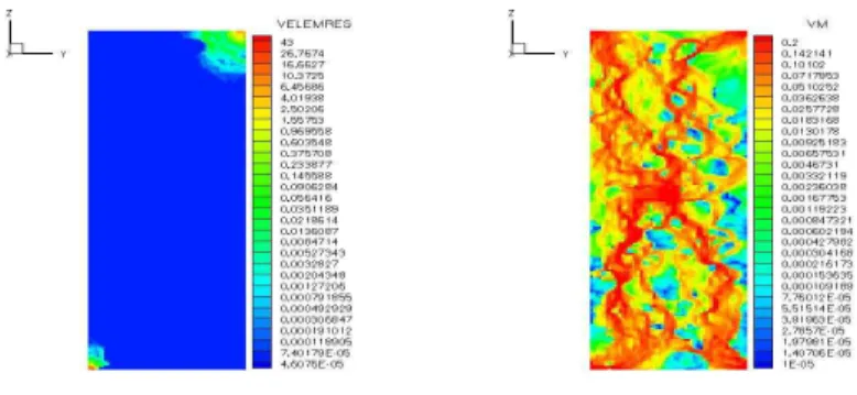
6. Numerical results

In this section we present numerical results for some benchmark problems [18]. In particular we consider two problems: the idealized diagonal channel problem and the fluvial reservoir problem (85th layer of the 10th SPE compar- ative project), that were previously studied for incompressible flow by Aarnes et al. by applying several multiscale mixed methods. Similar solutions were obtained using mortars and they compared favorably. The solutions shown here are of log |u| for slightly compressible flow. A fluid compressibility factor of 4.0E-05 was assumed. All computations were run in parallel on up to 16 processors at the beowulf cluster in the Center for Subsurface Modeling at the University of Texas at Austin.

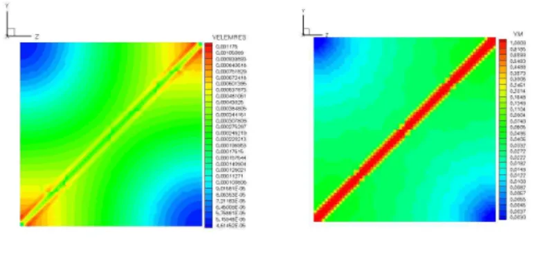
6.1. Diagonal Channel

This problem has proved quite challenging to most multiscale methods.

Here, a single high-permeability channel goes diagonally from the source to the sink. The domain is a square 64m × 64m × 1m. The permeability is 100 times as high along the diagonal as it is elsewhere. A unit source and unit sink are located at either ends of the high-permeable layer (which is 3 elements thick, away from the boundary). The domain is partitioned into 64 subdo- mains (8 × 8 coarse mesh). Each subdomain is further sub-divided into an 8 × 8 fine-mesh (giving a fine element size of 1m × 1m).

The Figure 1 shows the reference solution on the left, on a single-domain

(64m × 64m fine mesh) and the mortar solution on the right on an 8 × 8

subdomain partition. Further, we find that by applying a posteriori error esti-

mates loosely based on [31], the mortar degrees of freedom can be chosen to be

coarser away from the regions where the error in the solution is higher, while

VM 1.0000E-00 8.1847E-01 6.6990E-01 5.4829E-01 4.4876E-01 3.6730E-01 3.0062E-01 2.4605E-01 2.0139E-01 1.6483E-01 1.3491E-01 1.1042E-01 9.0375E-02 7.3970E-02 6.0542E-02 4.9552E-02 4.0557E-02 3.3195E-02 2.7169E-02 2.2237E-02 1.8201E-02 1.4897E-02 1.2192E-02 9.9792E-03 8.1677E-03 6.6850E-03 5.4715E-03 4.4783E-03 3.6654E-03 3.0000E-03

VM 1.0000E+00 8.1847E-01 6.6990E-01 5.4829E-01 4.4876E-01 3.6730E-01 3.0062E-01 2.4605E-01 2.0139E-01 1.6483E-01 1.3491E-01 1.1042E-01 9.0375E-02 7.3970E-02 6.0542E-02 4.9552E-02 4.0557E-02 3.3195E-02 2.7169E-02 2.2237E-02 1.8201E-02 1.4897E-02 1.2192E-02 9.9792E-03 8.1677E-03 6.6850E-03 5.4715E-03 4.4783E-03 3.6654E-03 3.0000E-03

Figure 1. Diagonal channel: Reference and mortar solutions.

preserving the accuracy of the solution. These are shown in Figure 2 on a 4 × 4 coarse mesh partitioning.

Figure 2. Diagonal channel: Residual based errors and coarse-mortar solution.

6.2. Fluvial Reservoir

As a second example, we considered a more realistic fluvial reservoir prob- lem, where the permeability field contains many narrow high flow “channels”.

This permeability data was taken from Layer 85 of the 10th SPE Comparative Project [9]. For comparison purposes, although the true measurements are in feet, the solution was calculated in SI units as in [18]. The fine mesh consisted of 60 × 220 elements. Sources and sinks are placed in a five-spot pattern, with a unit source in the middle and sinks of strength 1/4 each at the four corners.

The true (reference) solution and the solution on a 5 × 11 coarse mesh (55

subdomains) using mortars are shown in Figures 3 and 4. The mortar degrees

of freedom were again chosen coarse where the errors were small. The errors

were highest at the bottom-left and top-right corners of the domain because of

the very low permeability, yet equal flow rates at the sinks in these corners.

Figure 3. Fluvial Reservoir: Permeability and reference solution.

Figure 4. Fluvial Reservoir: Residual-based errors and coar- se mortar solution.

7. Conclusion

Multiscale mortar mixed finite element method [2] has been extended to a nonlinear parabolic problem. Both theoretical error estimates and computa- tional results on multiscale benchmark problems have been presented. These computational examples, especially for compressible flows, have proven chal- lenging for emerging multiscale algorithms. Our simulation results are among the first to have been performed on a parallel cluster.

A posteriori error estimators for the mortar spaces have been applied in the computations. Details of this work including analysis and parallel scalability will appear in a future paper.

Acknowledgments. Much of this work was done while the first and second

authors were visiting ICES, The University of Texas at Austin. They would

like to thank for the hospitality and support via the J. Tinsley Oden Faculty Fellowship Program during the visit.

References

[1] T. Arbogast, L. C. Cowsar, M. F. Wheeler, and I. Yotov, Mixed finite element methods on nonmatching multiblock grids, SIAM J. Numer. Anal. 37 (2000), no. 4, 1295–1315.

[2] T. Arbogast, G. Pencheva, M. F. Wheeler, and I. Yotov, A multiscale mortar mixed finite element method, Technical Report TR-MATH 06-15, Department of Mathematics, University of Pittsburgh, 2006, Submitted to Multiscale Model. Simul.

[3] J. Bear, Dynamics of Fluids in Porous Media, Dover Publication, Inc. New York, 1988.

[4] C. Bernardi, Y. Maday, and A. T. Patera, A new nonconforming approach to domain decomposition: the mortar element method, Nonlinear partial differential equations and their applications. College de France Seminar, Vol. XI (Paris, 1989–1991), 13–51, Pitman Res. Notes Math. Ser., 299, Longman Sci. Tech., Harlow, 1994.

[5] F. Brezzi, J. Douglas, Jr., M. Fortin, and L. D. Marini, Efficient rectangular mixed finite elements in two and three space variables, RAIRO Model. Math. Anal. Numer.

21 (1987), no. 4, 581–604.

[6] F. Brezzi, J. Douglas, Jr., and L. D. Marini, Two families of mixed finite elements for second order elliptic problems, Numer. Math. 47 (1985), no. 2, 217–235.

[7] F. Brezzi and M. Fortin, Mixed and hybrid finite element methods, Springer Series in Computational Mathematics, 15. Springer-Verlag, New York, 1991.

[8] Z. Chen and T. Y. Hou, A mixed multiscale finite element method for elliptic problems with oscillating coefficients, Math. Comp. 72 (2003), no. 242, 541–576.

[9] M. A. Christie and M. J. Blunt, Tenth SPE comparative solution project: A comparison of upscaling techniques, SPE Reservoir Eval. Eng. 4 (2001), no. 4, 308–317.

[10] L. C. Cowsar, J. Mandel, and M. F. Wheeler, Balancing domain decomposition for mixed finite elements, Math. Comp. 64 (1995), no. 211, 989–1015.

[11] J. Douglas, Jr., R. E. Ewing, and M. F. Wheeler, The approximation of the pressure by a mixed method in the simulation of miscible displacement, RAIRO Anal. Numer. 17 (1983), no. 1, 17–33.

[12] J. Douglas, Jr. and J. E. Roberts, Global estimates for mixed methods for second order elliptic equations, Math. Comp. 44 (1985), no. 169, 39–52.

[13] R. Dur´ an, Superconvergence for rectangular mixed finite elements, Numer. Math. 58 (1990), no. 3, 287–298.

[14] R. E. Ewing, R. D. Lazarov, and J. Wang, Superconvergence of the velocity along the Gauss lines in mixed finite element methods, SIAM J. Numer. Anal. 28 (1991), no. 4, 1015–1029.

[15] R. Glowinski and M. F. Wheeler, Domain decomposition and mixed finite element meth- ods for elliptic problems, First International Symposium on Domain Decomposition Methods for Partial Differential Equations (Paris, 1987), 144–172, SIAM, Philadelphia, PA, 1988.

[16] P. Grisvard, Elliptic problems in nonsmooth domains, Monographs and Studies in Math- ematics, 24. Pitman (Advanced Publishing Program), Boston, MA, 1985.

[17] M.-Y. Kim, F. A. Milner, and E.-J. Park, Some observations on mixed methods for fully nonlinear parabolic problems in divergence form, Appl. Math. Lett. 9 (1996), no.

1, 75–81.

[18] V. Kippe, J. E. Aarnes, and K.-A. Lie, Multiscale finite-element methods for elliptic problems in porous media flow, Multiscale Model. Simul., (2006, to appear).

[19] T. P. Mathew, Domain decomposition and iterative refinement methods for mixed finite

element discretizations of elliptic problems, PhD thesis, Courant Institute of Mathemat-

ical Sciences, New York University, 1989.

[20] F. A. Milner and E.-J. Park, A mixed finite element method for a strongly nonlinear second-order elliptic problem, Math. Comp. 64 (1995), no. 211, 973–988.

[21] M. Nakata, A. Weiser, and M. F. Wheeler, Some superconvergence results for mixed finite element methods for elliptic problems on rectangular domains, The mathematics of finite elements and applications, V (Uxbridge, 1984), 367–389, Academic Press, London, 1985.

[22] J. C. Ned´el´ec, Mixed finite elements in R ³ , Numer. Math. 35 (1980), no. 3, 315–341.

[23] E.-J. Park, Mixed finite element methods for nonlinear second-order elliptic problems, SIAM J. Numer. Anal. 32 (1995), no. 3, 865–885.

[24] , Mixed finite element methods for generalized Forchheimer flow in porous media, Numer. Methods Partial Differential Equations 21 (2005), no. 2, 213–228.

[25] P. A. Raviart and J. M. Thomas, A mixed finite element method for 2nd order elliptic problems, Mathematical aspects of finite element methods (Proc. Conf., Consiglio Naz.

delle Ricerche (C.N.R.), Rome, 1975), pp. 292–315. Lecture Notes in Math., Vol. 606, Springer, Berlin, 1977.

[26] J. E. Roberts and J. M. Thomas, Mixed and hybrid methods, Handbook of numerical analysis, Vol. II, 523–639, Handb. Numer. Anal., II, North-Holland, Amsterdam, 1991.

[27] T. Russell and M. F. Wheeler, Finite element and finite difference methods for continu- ous flows in porous media in The Mathematics of Reservoir Simulation, R. E. Ewing, ed., Frontiers in Applied Mathematics 1, Society for Industrial and Applied Mathematics, Philadelphia, 1984, pp. 35–106.

[28] L. R. Scott and S. Zhang, Finite element interpolation of nonsmooth functions satisfying boundary conditions, Math. Comp. 54 (1990), no. 190, 483–493.

[29] A. Weiser and M. F. Wheeler, On convergence of block-centered finite differences for elliptic problems, SIAM J. Numer. Anal. 25 (1988), no. 2, 351–375.

[30] M. F. Wheeler, A priori L 2 error estimates for Galerkin approximations to parabolic partial differential equations, SIAM J. Numer. Anal. 10 (1973), 723–759.

[31] M. F. Wheeler and I. Yotov, A posteriori error estimates for the mortar mixed finite element method, SIAM J. Numer. Anal. 43 (2005), no. 3, 1021–1042.

[32] I. Yotov, Mixed finite element methods for flow in porous media, PhD thesis, Rice University, Houston, Texas, 1996, TR96-09, Dept. Comp. Appl. Math., Rice University and TICAM report 96-23, University of Texas at Austin.

Mi-Young Kim

Department of Mathematics Inha University

Incheon 402-751, Korea

E-mail address: [email protected]

Eun-Jae Park

Department of Mathematics Yonsei University

Seoul 120-749, Korea

E-mail address: [email protected]

Sunil G. Thomas

Institute for Computational Engineering and Sciences The University of Texas at Austin

Austin, TX 78712

E-mail address: [email protected]

Mary F. Wheeler

Institute for Computational Engineering and Sciences Department of Aerospace Engineering Mechanics

and Department of Petroleum and Geosystems Engineering The University of Texas at Austin

Austin, TX 78712

E-mail address: [email protected]