* ㈜삼성중공업 선박해양연구센터 (교신저자)
** ㈜삼성중공업 선박해양연구센터 E-mail : [email protected]
DOI : https://www.doi.org/10.33519/kwea.2021.12.3.005 Received : May 26, 2021, Revised : September 3, 2021, Accepted : September 10, 2021
1. Introduction
With the Korea’s Renewable Energy 2030 plan, the Korean government announced a plan to in- crease in the proportion of renewable energy development to 20 % by 2030. One way to achieve this is a large floating offshore wind turbine
풍력에너지저널 pp. 32~44
부유식해상풍력 용 동해가스전 환경조건1)
최용호*․김현조**
Environmental Conditions of Donghae Gas Field for FOWT
Yong-Ho Choi* and Hyun-Joe Kim**
Key Words : Floating offshore wind turbine (부유식해상풍력터빈), Design load case (설계하중조건),
National oceanic and atmospheric administration (미국해양대기청), Hybrid coordinate ocean model (미국 고해상도 해양예보모형), Korea meteorological administration (한국기상청)
ABSTRACT
This paper aims to estimate the design values of environmental conditions such as wind, waves, and sea current in the Donghae gas field for the floating offshore wind turbine (FOWT) design specified in the IEC 61400 standard. In this paper, 39-year National Oceanic and Atmospheric Administration (NOAA) long-term hindcast data and 3-year Korea Meteorological Administration (KMA) buoy measured data were used for wind and waves, while 22-year HYbrid Coordinate Ocean Model (HYCOM) data were used for sea currents. The generalized Pareto distribution (GPD), 3-parameter Weibull distribution (W3P) and inverse first order reliability method (IFORM) recommended by DNVGL were used for extreme value analyses. In particular, for significant wave heights of severe sea state (SSS) required in the design load case (DLC) 1.6, it was found that the fitting method recommended by the International Electrotechnical Commission (IEC) was not suitable for these data sets. Therefore, this paper proposes to use a different method to obtain appropriate values. The environmental conditions presented in this study are expected to be useful information for FOWT design and substations to be installed and operated in the Donghae gas field in the future.
Nomenclature : spectral peak wave period (s)
: sea current speed (m/s)
: year return period (year)
: recording interval
: mean wind speed (m/s)
: mean wind speed at the height of hub (m/s)
: significant wave height (m)
(FOWT), which can be considered for Donghae gas field, and could also be a strong candidate.
Unfortunately, however, there are no well-organized environmental data such as wind, wave, and sea current data for the site. Therefore, this study aims to estimate design environmental conditions for reduced design load cases (DLCs) defined by IEC 61400-1 [1], 61400-3-1 [2], and 61400-3-2 [3] using 39-year National Oceanic and Atmospheric Admini- stration (NOAA) long-term hindcast data for wind and wave and 22-year HYCOM data for water level and sea current. The extreme values of the 3-year Korea Meteorological Administration (KMA) [4]
measurement by buoy for wind and wave were used to be compared with the results from NOAA. This study also provides the contemporaneous significant wave height (Hs) with the mean wind speed at the height of the hub from the still water level () required by normal sea state (NSS) and severe sea state (SSS).
2. Database and Analysis Method
2.1 KMA, NOAA, HYCOM data of Donghae gas field
The location of the Donghae gas field is shown in Fig. 1. The KMA weather buoy near the Donghae gas field is located at Ulsan 22189 with Lat.34.45N and Lon.129.47E. The 3-year KMA buoy data were measured from 1st January 2016 to 1st January 2019. The KMA data provide 10-minute average wind speeds at 4.3m above the calm water level, 4.3m-10min-Vw (m/s). The wave of KMA
data consist of the 17-minute significant wave height, 17min-Hs (m), and the spectral peak wave period, Tp (s), for about 17 minutes with 1 Hz of sampling rate and 1,024 samples for Fourier transform. There are three kinds of recording intervals (RIs), which are 30 minutes, 1 hour and 1 day. The 39-year (from 1st January 1979 to 31st December 2017) NOAA long-term hindcast data were also used for the extreme value analysis for Lat. 35.5N and Lon. 130.0E at the mean water depth of 150 m. The NOAA data consist of the significant wave height over 3 hours, 3hr-Hs, and Tp, and 1-hour averaged wind speed at the height of 10m, 10m-1hr-Vw, with 3-hour recording interval. The 22-year (from 1st January 1994 to 31st December 2015) HYbrid Coordinate Ocean Model (HYCOM) data were considered in the extreme value analysis for the sea current for Lat. 35.52N and Lon. 130.0E.
source. These are summarized in Table 1. This table also shows the number of data.
Table 1 Database
KMA NOAA HYCOM
source buoy measurement hindcast hindcast
gathering 1Hz,
1024 samples simulation by
NOAA model Reanalysis by HYCOM
RI 30min, 1hr, 1day 3hr 3hr
output 4.3m-10min-Vw
17min-Hs/Tp 10m-1hr-Vw
3hr-Hs/Tp sea level sea current no. data 48672: 3yr, 30min 113933: 39yr 63341: 22yr
Table 2 50-year extreme conditions of Donghae gas field [5, 6]
Ref [5]: 10min-Vw at hub height (90 m)
period 8-years 39-years 3-years
source ECMWF-
ERA5 NASA-
MERRA-2 Ulasn NOMAD
weather buoy 50yr-90m-
10min-Vw 40.65m/s 40.69m/s 39.46m/s
Ref [6]: 3 years KMA measured buoy data
period 2016.01.01.-2019.01.01
50yr-90m-10min-Vw 39.83m/s
50yr-10m-1hr-Vw 29.06m/s converted by NPD wind profile 50yr-17min-Hs; Tpby Gumbel
fitting with Monthly 36 peaks 11.12m; 14.17s
current speed 0.163m/s
highest water level 0.7m
Fig. 1 Location of Donghae gas field [5]
2.2 Previous studies for wind, wave and current Despite the lack of reliable environmental data for the Donghae site, 50-year return period extreme conditions as shown in Table 2 have been obtained thanks to Shin's previous studies [5, 6]. For unclear definitions in the reference [6], we contacted KMA for confirmation, and the results are shown in red letters in the table. The blue letters in the table show wind speeds converted using NPD wind profile.
2.3 Analysis methods
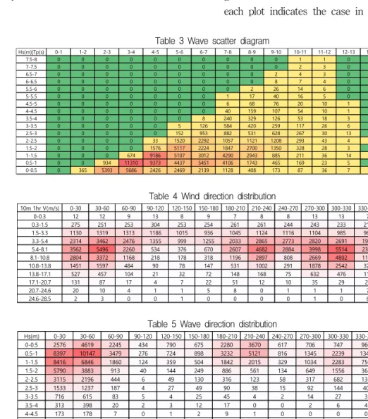
The extreme value theory (EVT) was considered in this study [7-12]. The generalized Pareto distri- bution (GPD) and 3-parameter Weibull distribution for the highest 10 % of the data (hereafter W3P) were used for extreme value analyses for the wind data. While GPD and W3P as well as inverse first order reliability method (IFORM) approach recommended by DNVGL-RP-C205 were used for the wave data. The kernel density estimation (KDE) approach as a non-parametric method was also examined. In order to check the goodness-of-fit, the Kolmogorov–Smirnov test (K-S test) statistics are given in the GPD and W3P fitting plots. A “tie” in each plot indicates the case in which the data have Table 3 Wave scatter diagram
Hs(m)|Tp(s) 0-1 1-2 2-3 3-4 4-5 5-6 6-7 7-8 8-9 9-10 10-11 11-12 12-13 13-14 14-15
7.5-8 0 0 0 0 0 0 0 0 0 0 1 1 0 0 0
7-7.5 0 0 0 0 0 0 0 0 0 0 2 3 0 0 0
6.5-7 0 0 0 0 0 0 0 0 0 2 4 3 0 0 0
6-6.5 0 0 0 0 0 0 0 0 0 8 7 4 0 0 0
5.5-6 0 0 0 0 0 0 0 0 2 26 14 6 0 0 0
5-5.5 0 0 0 0 0 0 0 1 17 40 16 5 0 0 0
4.5-5 0 0 0 0 0 0 0 6 68 76 20 10 1 0 0
4-4.5 0 0 0 0 0 0 0 40 159 107 54 10 1 0 0
3.5-4 0 0 0 0 0 0 8 240 329 126 53 18 3 0 0
3-3.5 0 0 0 0 0 5 126 584 420 259 117 26 6 0 0
2.5-3 0 0 0 0 0 152 953 882 531 628 267 30 13 0 0
2-2.5 0 0 0 0 33 1520 2292 1057 1121 1208 293 43 4 1 0
1.5-2 0 0 0 0 1576 5117 2224 1847 2700 1350 328 28 3 0 0
1-1.5 0 0 0 674 9186 5107 3012 4290 2943 885 211 36 14 3 1
0.5-1 0 0 934 11310 9373 4437 5451 4106 1743 465 169 23 5 0 0
0-0.5 0 365 5393 5686 2426 2469 2139 1128 408 173 87 36 7 3 0
Table 4 Wind direction distribution
10m 1hr V(m/s) 0-30 30-60 60-90 90-120 120-150 150-180 180-210 210-240 240-270 270-300 300-330 330-360 Freq.(%)
0-0.3 12 12 9 13 8 9 7 8 8 13 13 7 0.10%
0.3-1.5 275 251 253 304 253 254 261 261 244 243 233 216 2.68%
1.5-3.3 1130 1319 1313 1186 1015 936 1045 1124 1116 1104 985 962 11.64%
3.3-5.4 2314 3462 2476 1355 999 1255 2033 2865 2773 2820 2691 1923 23.71%
5.4-8.1 3562 5496 2260 534 376 670 2607 4682 2884 3998 5514 2388 30.74%
8.1-10.8 2804 3372 1168 218 178 318 1196 2897 808 2669 4802 1196 19.01%
10.8-13.8 1451 1597 484 90 78 147 531 1002 291 1878 2542 370 9.20%
13.8-17.1 527 457 104 21 32 72 148 168 75 632 476 113 2.48%
17.1-20.7 131 87 17 4 7 22 51 12 10 35 29 23 0.38%
20.7-24.6 20 10 4 1 1 5 8 0 1 1 1 7 0.05%
24.6-28.5 2 3 0 0 1 0 0 0 0 1 0 6 0.01%
Table 5 Wave direction distribution
Hs(m) 0-30 30-60 60-90 90-120 120-150 150-180 180-210 210-240 240-270 270-300 300-330 330-360 Freq.(%)
0-0.5 2576 4619 2245 434 790 675 2280 3670 617 706 747 960 17.83%
0.5-1 8397 10147 3479 276 724 898 3232 5121 816 1345 2239 1342 33.37%
1-1.5 8416 6846 1860 124 359 504 1842 2015 329 1034 2283 750 23.14%
1.5-2 5790 3883 913 40 144 249 886 561 134 649 1556 368 13.32%
2-2.5 3115 2196 444 6 49 130 316 123 58 317 682 136 6.65%
2.5-3 1533 1237 187 4 27 49 90 38 15 92 144 40 3.03%
3-3.5 716 615 83 5 4 25 45 4 2 14 27 3 1.35%
3.5-4 313 398 20 2 3 12 17 0 0 2 6 4 0.68%
4-4.5 173 178 7 0 1 2 9 1 0 0 0 0 0.33%
4.5-5 69 92 9 0 2 3 5 1 0 0 0 0 0.16%
5-5.5 38 37 0 0 0 0 2 0 0 0 0 2 0.07%
5.5-6 22 25 0 0 0 0 0 0 0 0 0 1 0.04%
6-6.5 9 10 0 0 0 0 0 0 0 0 0 0 0.02%
6.5-7 4 5 0 0 0 0 0 0 0 0 0 0 0.01%
7-7.5 2 3 0 0 0 0 0 0 0 0 0 0 0.00%
7.5-8 1 1 0 0 0 0 0 0 0 0 0 0 0.00%
the same value. For large sample size, the tie can be ignored, otherwise, the null hypothesis cannot be rejected if the value of the K-S test statistic, D, is small. Q-Q plots are also shown in the GPD fitting.
3. Extreme Value Analysis
3.1 Wind and wave by 39-year NOAA hind- cast data
The 39-year NOAA long-term hindcast data were used in the extreme value analysis (EVA) for the Donghae gas field, S. Korea (Lat. 35.5N and Lon. 130.0E). Table 3 shows the frequency distribution of Hs and Tp. Table 4 and 5 show the distribution of the coming-from wind and wave directions, respectively.
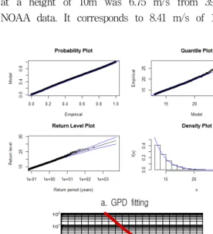
3.1.1 Extreme marginal wind
An average value of all 1 hour mean wind speeds at a height of 10m was 6.75 m/s from 39-year NOAA data. It corresponds to 8.41 m/s of 128m-
10min–Vw by the NPD (Norwegian Petroleum Directorate, ISO) wind profile [13]. Fig. 2 represents the GPD of EVA and W3P fittings with the threshold value of 13 m/s by R and in-house code, respectively.
3.1.2 Extreme marginal sea states with Hs and Tp
Fig. 3 shows the scatter plot of Hs and Tp. As per DNVGL [13], IFORM with conditional modelling approach (CMA) was used to construct extreme environmental contours. According to CMA, a joint probability distribution of Hs and Tp is separated into a marginal distribution of Hs and a conditional distribution of Tp on each Hs. Then the data are fitted to these two distributions. Fig. 4 shows the
a. GPD fitting
Vw [m/s]
1-CDF[%]
0 10 20 30 40
10-4 10-3 10-2 10-1 100 101 102
W3P Extreme Values:
Shape=0.98050 SScale=1.74366 SLocation=13.06492
b. W3P fitting
Fig. 2 GPD and W3P fittings for wind speeds for NOAA data.
a: threshold=13m/s, n(POT)=5047, D=0.0166, p-value=0.4867, tie.
b: threshold=13m/s, n(POT)=4885, D=0.0358, p-value=0.0038, tie.
Fig. 3 Scatter plot of Hs-Tp for 39-year NOAA data
Given Fitted
ln(H-shift)
-0.29 0.22 0.56 0.81 1.18 1.451.75 1.98
ln(ln(1/(1-F)))
2.00 1.50 1.00 0.50 0.00
Given Fitted
Hs[m]
0.25 2.25 4.25 6.25 8.25 10.75 13.25 15.75 18.25
Mean lnT
2.00
1.00
0.00
Given Fitted
Hs[m]
0.25 2.25 4.25 6.25 8.25 10.75 13.25 15.75 18.25
Var lnT
0.20 0.15 0.10 0.05 0.00
Tp(s)
Hs(m)
0 2 4 6 8 10 12 14 16 18 20 2224
0 1 2 3 4 5 6 7 8 9 10
Median sqrt(15Hs) 5%CI 95%CI 1yr 10yr 50yr
Fig. 4 IFORM approach for 39-year NOAA data
IFORM results of Hs and Tp.
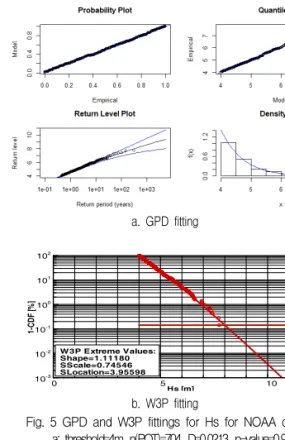
Fig. 5 shows the GPD fitting with the threshold value of 3m of Hs and W3P fitting with the threshold value of 4m of Hs. Fig. 6 shows the KDE environmental contour by R. Since the KDE contour, however, highly depends on the kernel width and has no proper method to select a suitable width, the KDE approach was not applied to estimate the design extreme values in this present study.
3.1.3 Results of extreme value analysis
Table 6 summarizes the extreme values of the 39-year NOAA data for the Donghae gas field. This table also shows the converted wind speeds for different average time intervals, different reference heights such as 100 m and 128 m, and different definitions of wind profiles. For the design of wind turbine, a conversion factor of 0.95 from 1hr-Vw to 10min-Vw as per IEC 61400-3-1:2019, and 0.11 of exponent of power wind profile for the extreme wind speed model (EWM) as per IEC 61400-1:2019 were used. The wind speeds converted by the NPD wind profile are also useful to use commercial software such as Orcaflex or SIMA of DNV to generate turbulence wind field for the design of floating supporting sub-structure and the station- keeping mooring. Interestingly, the wind speed converted by the IEC standard is almost the same as that of the NPD wind profile. Since all extreme values by IFORM, GPD and W3P for wave were similar with quite small differences, the highest values could be chosen as the extreme design values. This table also shows the 90 % confidence intervals of Tp using the 5th and 95th percentiles which may be used for Tp sensitivity tests. 29.04 m/s of 50-year 10m-1hr-Vw in this table is approximately equal to 29.06 m/s in Table 2 of the previous study. For reference, reliable wind data from NOAA, CFSR(Climate Forecast System Reanalysis, USA), ERA5(ECMWF ReAnalysis v5) and MERRA-2(Modern Era Retrospective analysis for Research and Applications v2) are provided free of charge. Moreover, NOAA's wind data is based on CFSR. From Tables 1 and 5, it can be seen that 50-YRP extreme wind speed from NOAA is similar to the values of ERA5, MERRA-2, and KMA.
Therefore, it can be said that the difference between the sources of wind data is negligible for the Donghae gas field. The results in Table 6 require verification using at least 30 years field measurements. However, the actual measurements so far have only been measured for 3 years by the KMA, which is insufficient for verification. Although not mentioned in this paper, a 50-year 3hr sea state was separately estimated based on ECMWF's 42.4 years ERA5 data (1979.01.01-2021.04.30, European a. GPD fitting
Hs [m]
1-CDF[%]
0 5 10
10-3 10-2 10-1 100 101 102
W3P Extreme Values:
Shape=1.11180 SScale=0.74546 SLocation=3.95598
b. W3P fitting
Fig. 5 GPD and W3P fittings for Hs for NOAA data a: threshold=4m, n(POT)=704, D=0.0213, p-value=0.9972, tie b: threshold=4m, n(POT)=704, D=0.0526, p-value=0.2853, tie
Fig. 6 KDE environmental contour for Hs for NOAA data
Center for Medium-Range Weather Forecasts). As a result, 3hr-Hs=8.24m and Tp=11.79s were obtained, which confirmed that there was only a difference of 1.5% from the values in Table 6.
An assumption of a zero-mean Gaussian random process of wave gives the Rayleigh distribution of wave heights. Then, the maximum design regular wave for the 50-year extreme sea state with 3hr-Hs=8.12m and Tp=11.50s in Table 6 is about 15.39m. Here, a fully-developed sea is assumed to
convert Tp to Tz.
3.1.4 Wind speeds versus significant wave heights Fig. 7 and Table 7 show the scatter plot of 1-hour average wind speed at a height of 10 m, 10m-1hr–Vw, and 3hr-Hs.
Table 8 NSS conditional on normal wind conditions for 39-year NOAA data of Donghae gas field 10m-1hr
Vw(m/s) Mean Hs(m)
IEC standard NPD wind profile 10m-10min
Vw(m/s) 128m-10min
Vw(m/s) 128m-10min Vw(m/s)
1 0.63 1.05 1.50 1.19
3 0.65 3.16 4.51 3.63
5 0.80 5.26 7.52 6.15
7 1.08 7.37 10.53 8.74
9 1.44 9.47 13.54 11.40
11 1.83 11.58 16.55 14.12
13 2.23 13.68 19.55 16.90
15 2.72 15.79 22.56 19.74
17 3.31 17.89 25.57 22.62
19 3.97 20.00 28.58 25.56
21 4.65 22.11 31.59 28.55
23 4.94 24.21 34.60 31.59
25 5.08 26.32 37.60 34.68
27 6.50 28.42 40.61 37.81
Table 6 Summary of the extreme values of the wind turbine for 39-years NOAA data of Donghae gas field
Analysis Method
Wave Wind speed Vw (m/s)
from NOAA data IEC standard NPD wind profile
Thre- shold Hs
(m) Tp(s) 5% Tp(s)
Median Tp(s) 95% Thre-
shold 10m-
1hr 10m-
10min 100m-10min
alpha=0.11 128m-10min alpha=0.11 100m-
10min 128m- 10min
Given 7.74 Given 27.84 29.31 37.75 38.79 38.31 39.14
IFORM
39yr 7.98 10.67 11.42 12.21
1yr 5.85 8.90 10.06 11.37
5yr 6.80 9.73 10.69 11.74
10yr 7.20 10.06 10.94 11.90
50yr 8.12 10.78 11.50 12.27
GPD 39yr
4.0m 7.98
13m/s
27.79 29.26 37.69 38.73 38.23 39.09
1yr 5.91 21.67 22.82 29.39 30.20 28.98 29.57
5yr 6.86 24.41 25.69 33.10 34.01 33.07 33.76
10yr 7.25 25.56 26.91 34.66 35.62 34.81 35.55
50yr 8.11 28.20 29.68 38.24 39.29 38.87 39.72
3-p Weibull for high exceedances
39yr 4.0m
8.00
13m/s
28.58 30.08 38.76 39.82 39.46 40.32
1yr 5.89 21.81 22.96 29.58 30.39 29.19 29.78
5yr 6.84 24.78 26.08 33.60 34.53 33.63 34.34
10yr 7.24 26.06 27.43 35.34 36.31 35.58 36.34
50yr 8.14 29.04 30.57 39.38 40.46 40.17 41.07
Table 7 Wind-wave scatter diagram for NOAA data of Donghae gas field
Hs:1hr 10m V 0-2 2-4 4-6 6-8 8-10 10-12 12-14 14-16 16-18 18-20 20-22 22-24 24-26 26-28
7-8 0 0 0 0 0 0 0 0 0 2 0 2 1 2
6-7 0 0 0 0 0 0 0 1 6 7 9 1 2 2
5-6 0 0 0 0 0 5 9 28 36 23 16 6 2 2
4-5 0 0 0 13 32 69 117 139 94 50 28 6 4 0
3-4 4 11 41 141 275 516 599 424 216 73 15 2 3 0
2-3 83 281 708 1363 2201 2731 2220 1136 265 34 5 1 0 0
1-2 877 3156 6321 10165 11515 6871 2279 322 27 2 0 0 0 0
0-1 4810 15369 20328 13739 3669 387 32 2 0 0 0 0 0 0
Fig. 7 Scatter plot of 10m-1hr-Vw and 3hr-Hs for NOAA data of Donghae gas field
For the design of the wind turbine, floating supporting substructure and station-keeping mooring, wind and current as well as wave are to be defined.
The DLCs defined in IEC 61400-3-1:2019 and 61400-3-2:2019 recommend , which is the average Hs in normal sea state (NSS) conditional on the hub height 10-minute mean wind speed, Vhub. Table 8 shows the results using the 39 years NOAA data. In this study, unlike the 90 m in Table 2, the hub height was assumed to be 128 m above the mean water level. For the design of wind turbine, the conversion factor of 0.95 and 0.14 of exponent for the normal wind conditions were applied as per the IEC standard. For the design of floating supporting sub-structure and station-keeping mooring, the NPD wind profile was used to convert the wind speeds. In Table 8, the NPD wind profile yields slightly more conservative mean Hs for the 128m-10min-Vw than the IEC standard wind profile.
For conditional extreme Hs, contour analysis was carried out to estimate extreme seastates to be used for mooring analysis along extreme contour lines. As per IEC 61400-3-1:2019, IFORM with CMA was used in the environmental contour analysis. The W3P distribution was used for the marginal distribution of 10m-1hr-Vw, Hs|Vw. First of all, the normal and log-normal conditional Hs distributions for the given mean wind speed recommended by IEC were checked. Fig. 8-a and b show the contours for 50-year return period (YRP) obtained using normal and log-normal conditional Hs distributions, respectively. This figure shows
that the normal and log-normal conditional distributions in this case are not appropriate for the joint probability consisting of Vw and Hs.
On the other hand, the so-called wave-Height- conditional-on-wind-Speed (HCW) approach was applied to Vw and Hs, with W3P distribution of Hs for the design of the substructure and mooring analyses. According to this HCW approach, the extreme Hs’s conditional on the 10m-1hr-Vw’s for 1-YRP and 50-YRP were estimated as shown in Fig. 9. The HCW contours show good estimations of 1-YRP and 50-YRP contours for the extreme Hs’s conditional on the 10m-1hr-Vw’s for the range of operating wind speeds at hub height from cut-in, Vin, to cut-out, Vout, wind speeds. Applying Vin of 4 m/s and Vout of 25 m/s at the hub height of 128 m, the wind speed range of 10m height becomes 3.02m/s to 18.89m/s based on 0.11 of the power law for the EWM. Thus, the contours obtained by the HCW approach cover the range of wind speeds at a height of 10 m.
The extreme Hs’s conditional on the 128m- 10min-Vw’s were estimated from the results above as shown in Table 9. For the design of the wind turbine according to the IEC standard, the conver- sion between 1hr-Vw and 10min-Vw was carried out by applying a factor of 0.95 as per IEC 61400-3-1:2019. The wind speeds at different reference heights for the EWM were calculated using a power law with a power exponent of 0.11.
On the other hand, for the structure and mooring system, the NPD wind profile was used to convert
a. normal b. log-normal
Fig. 8 50-YRP contour of 10m-1hr-Vw and 3hr-Hs by IEC 61300-3-1 for 39-year NOAA data of Donghae gas field
with normal and log-normal conditional Hs distributions Fig. 9 50-YRP contours of Vw and Hs for 39-year NOAA data of Donghae gas field by HCW approach
the wind speed. This table shows similar Hs’s for the 128m-10min-Vw’s between two wind profiles.
3.2 Wind and wave by 3-year KMA data In this section, the statistics from the 39-year NOAA hindcast data will be compared with those from the 3-year buoy-measured KMA data.
3.2.1 All data
For wave data, EVA of the 3-year KMA wave data was carried out by IFORM, GPD and W3P fittings as shown in Fig. 10. Among them, IFORM with the method of moments (MOM) was the best fit. Table 10 summarizes the results of the extreme wave conditions estimated from the 3-year KMA data with 30 minutes and 1 hour of recording interval (RI) with 13 minutes and 43 minutes of idling time, respectively. In this table, there is no significant statistical difference between the recording intervals. DNV-OS-J101:2014 recommends a conversion factor of 1.09 from 3hr-Hs to 1hr-Hs with the assumption of a Rayleigh distribution and a number of waves of 1000 over 3 hours without any explanation. Applying its reciprocal value of 91.7 % to 17min-Hs’s in this table obtained from the 3-year KMA buoy-measured data near the Donghae gas field with a recording interval of 1-hour, 7.35 m and 8.13 m of 3hr-Hs’s for 10-YRP and 50-YRP were obtained, respectively. These values are approxi- mately equal to 7.24 m and 8.14 m in Table 6 obtained from the 39-year NOAA data. Further work on the conversion factor between different recording intervals will be done in the future.
For wind data, the average of 4.3m-10min-Vw in
128m- 10min- Vw (m/s)
IEC standard ISO wind profile 10m-
10min- Vw (m/s)
10m-1hr -Vw (m/s)
50yr Hs (m)
1yr Hs (m)
10m-1hr -Vw (m/s)
50yr Hs (m)
1yr Hs (m)
3 2.27 2.15 4.26 2.96 2.49 4.32 3.03
5 3.78 3.59 4.49 3.23 4.10 4.58 3.32
7 5.29 5.02 4.75 3.49 5.66 4.90 3.63
9 6.80 6.46 5.09 3.80 7.20 5.23 3.93
11 8.31 7.89 5.37 4.04 8.70 5.54 4.18
13 9.82 9.33 5.68 4.29 10.18 5.87 4.44 15 11.33 10.77 6.01 4.53 11.64 6.13 4.66 17 12.84 12.20 6.21 4.73 13.07 6.33 4.81 19 14.35 13.64 6.41 4.84 14.49 6.60 4.90 21 15.86 15.07 6.74 4.97 15.88 6.99 4.82 23 17.38 16.51 7.28 4.71 17.26 7.29 4.68 25 18.89 17.94 7.33 4.46 18.62 7.64 3.72 Table 9 Extreme significant wave heights conditional on the
hub height 10min wind speeds
a. GPD fitting
Hs [m]
1-CDF[%]
0 5 10
10-4 10-3 10-2 10-1 100 101 102
W3P Extreme Values:
Shape=1.04150 SScale=0.80116 SLocation=2.27873
Tp(s)
Hs(m)
0 2 4 6 8 10 12 14 16 18 20 22 24
0 1 2 3 4 5 6 7 8 9 10
1yr 10yr 50yr
b. W3P fitting c. IFORM contour Fig. 10 Extreme value analysis for 3-year KMA 30-min
wave data
a: threshold=2m, n(POT)=6447, D=0.1188, p-value<2.2e-16, tie b: threshold=2m, n(POT)=6447, D=0.0948, p-value<2.2e-16, tie
YRP 3-year measured KMA data
RI=30-min RI=1-hr
17min-
Hs(m) 17min-
Tp(s) 17min-
Hs(m) 17min- Tp(s) 10-yr1-yr
50-yr
6.798.08 8.96
10.47 11.15 11.57
6.738.01 8.86
10.54 11.24 11.68 Table 10 Extreme wave conditions from 3-year KMA 30-min
and 1-hr wave data for Donghae gas field
the 3-year KMA wind data was 6.42 m/s.
According to the NPD wind profile, it corresponds to 6.81 m/s of 10m-1hr-Vw and 8.02 m/s of 128m-10min-Vw which is 4.6 % smaller than 8.41 m/s in the 39-year NOAA data in section 3.1.1.
Although both the GPD and W3P fittings gave underestimations for large wind speed as shown in Fig. 11, the GPD results were larger than W3P results. Hence, the GPD results were chosen as resultant values as shown in Table 11. Limited to this study, comparing 10m-1hr-Vws of 50-YRP in Table 11 obtained from the 3-year KMA data and Table 6 from the 39-year NOAA data, 24.88 m/s in Table 11 is 14 % smaller than 39.04 m/s in Table 6 due to the under-estimation of the GPD fitting. In order to improve the fit results, at least 10 or 20 years of data are desired.
Table 11 Extreme wind conditions from 3-year KMA wind data
YRP KMA
4.3m-10min-Vw(m/s) Calculated 10m-1hr-Vw(m/s) RI=30-min RI=1-hr Diff. RI=30-min RI=1-hr 10-yr1-yr
50-yr 21.55 23.81 25.15
20.72 23.01 24.36
3.9%3.4%
3.1%
21.36 23.57 24.88
20.54 22.79 24.11
3.2.2 Monthly 36 peaks
Based on the EVT, the GPDs used so far in the sections used numerous peaks over threshold (POT) with the appropriately high threshold value to obtain statistically independent data. And IFORM results were compared to the GPD results. However, in this section, generalized extreme value (GEV) distribution as one of the EVTs was tested. Prior to the GEV analysis, independence of the data should be verified. Typically the 1-year block maxima method is used to obtain independent data for GEV analysis. However, in this section, monthly 36 peak data were used for analysis, assuming independence without any proof. Fig. 12 shows the GEV fitting results for the moonthly maxima of 17min-Hs and 4.3m-10min- Vw data with 30-min of RI. As can be seen from the figure, the 90 % confidence interval (CI) range for a long return period is extremely wider than that in Fig. 10 and Fig. 11.
a. 17min-Hs(m)
b. 4.3m-10min-Vw(m/s)
Fig. 12 GEV fittings for monthly 36 peaks for KMA 30-min wind a: n(data)=36, D=0.0833, p-value=0.9996, tie
b: n(data)=36, D=0.1100, p-value=0.9790, tie a. GPD fitting
Vw [m/s]
1-CDF[%]
0 10 20 30
10-4 10-3 10-2 10-1 100 101 102
W3P Extreme Values:
Shape=1.12075 SScale=1.94058 SLocation=10.65323
b. W3P fitting
Fig. 11 GPD fitting for 3-year KMA 30-min wind data a: threshold=10.7m/s, n(POT)=4717, D=0.0496, p-value=1.82e-05, tie b: threshold=10.7m/s, n(POT)=4717, D=0.0538, p-value=2.30e-06, tie
Table 12 shows the GEV analysis results with 90
% CI. Furthermore, regarding the GEV shape parameter, those for Hs and Vw were –0.028 and 0.073, respectively. Hence, Hs follows the Weibull distribution due to the negative shape parameter and Vw the Fréchet distribution due to the positive one, and Gumbel distribution is not appropriate in these cases. Using the Gumbel distribution to estimate extreme values for Hs and Vw data will lead to under- or over- estimated results. It has been pointed out that the Gumbel distribution can lead
their values to be considerably overestimated.
Moriarty et al. [14] suggest a W3P distribution to fit the extreme loads.
Fig. 13 shows the Gumbel fittings for the monthly maxima of 17min-Hs and 4.3m-10min-Vw data with 30-min of recording interval. Table 12 also shows the Gumbel fitting results. In the table, the 90 % CI of the value estimated by GEV are too wide to determine the design value due to the limited size of the data. The 50-YRP Hs and Vw by Gumbel are similar to those in Table 2 and are larger than the GEV results.
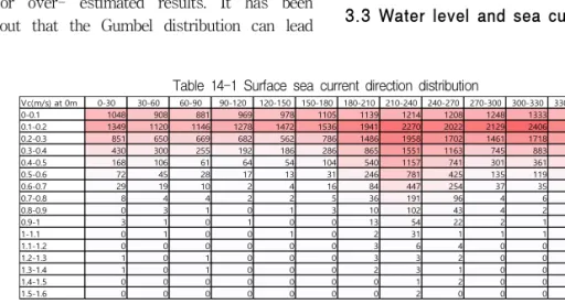
3.3 Water level and sea current
Table 14-1 Surface sea current direction distribution
Vc(m/s) at 0m 0-30 30-60 60-90 90-120 120-150 150-180 180-210 210-240 240-270 270-300 300-330 330-360 Freq.(%)
0-0.1 1048 908 881 969 978 1105 1139 1214 1208 1248 1333 1134 20.78%
0.1-0.2 1349 1120 1146 1278 1472 1536 1941 2270 2022 2129 2406 1913 32.49%
0.2-0.3 851 650 669 682 562 786 1486 1958 1702 1461 1718 1464 22.09%
0.3-0.4 430 300 255 192 186 286 865 1551 1163 745 883 866 12.19%
0.4-0.5 168 106 61 64 54 104 540 1157 741 301 361 421 6.44%
0.5-0.6 72 45 28 17 13 31 246 781 425 135 119 190 3.32%
0.6-0.7 29 19 10 2 4 16 84 447 254 37 35 58 1.57%
0.7-0.8 8 4 4 2 2 5 36 191 96 4 6 8 0.58%
0.8-0.9 0 3 1 0 1 3 10 102 43 4 2 0 0.27%
0.9-1 3 1 0 1 0 0 13 54 22 2 1 1 0.15%
1-1.1 0 1 0 0 1 0 2 31 1 1 1 1 0.06%
1.1-1.2 0 0 0 0 0 0 3 6 4 0 0 0 0.02%
1.2-1.3 1 0 1 0 0 0 3 3 2 0 0 0 0.02%
1.3-1.4 1 0 1 0 0 0 2 3 1 0 0 0 0.01%
1.4-1.5 0 0 0 0 0 0 0 1 2 0 0 0 0.00%
1.5-1.6 0 0 0 0 0 0 0 2 0 0 0 0 0.00%
Table 14-2 Sea current direction distribution at 60m below mean water level
Vc(m/s) at -60m 0-30 30-60 60-90 90-120 120-150 150-180 180-210 210-240 240-270 270-300 300-330 330-360 Freq.(%)
0-0.1 1599 1602 1880 2872 4273 3798 2935 2376 1693 1602 1600 1514 0.43801
0.1-0.2 1417 875 774 1534 3562 3231 4500 3409 1754 1206 1453 1890 0.404241
0.2-0.3 357 120 66 134 267 626 2287 1957 493 165 385 745 0.120017
0.3-0.4 17 17 1 9 20 103 637 825 142 19 20 42 0.029239
0.4-0.5 0 0 2 2 1 11 165 279 19 0 3 1 0.007625
0.5-0.6 0 0 0 0 0 0 24 29 1 0 0 0 0.000853
0.6-0.7 0 0 0 0 0 0 0 1 0 0 0 0 1.58E-05
Fig. 14 Water level for 22-year HYCOM data of Donghae
year Max (m) Min (m) Mean (m) year Max (m) Min (m) Mean (m)
1994 0.45 -0.002 0.197 2005 0.363 -0.163 0.163
1995 0.398 -0.025 0.183 2006 0.478 -0.083 0.160
1996 0.423 -0.1 0.174 2007 0.425 -0.094 0.161
1997 0.457 -0.09 0.206 2008 0.436 -0.099 0.159
1998 0.346 -0.028 0.175 2009 0.382 -0.057 0.177
1999 0.51 -0.062 0.195 2010 0.41 -0.081 0.184
2000 0.419 0.02 0.193 2011 0.441 -0.047 0.172
2001 0.414 0.005 0.207 2012 0.541 -0.025 0.203
2002 0.608 -0.057 0.183 2013 0.444 -0.054 0.197
2003 0.408 -0.036 0.172 2014 0.435 0.024 0.196
2004 0.434 -0.04 0.195 2015 0.487 -0.039 0.176
Table 13 Annual maxima, minima and average values of the water levels for 22-year HYCOM data of Donghae
YRP GEV Gumbel
17min-Hs(m) 4.3m-10min-Vw(m/s) 17min-
Hs(m) 4.3m-10min- Vw(m/s) 5% Med. 95% 5% Med. 95%
10-yr1-yr 50-yr
5.175.55 4.85
6.168.57 10.15
11.607.14 15.45
10.07 12.27 18.29
19.92 25.18 29.37
21.76 31.09 40.45
6.469.39 11.41
20.73 26.06 29.73 Table 12 Extreme values by GEV and Gumbel for monthly 36
peaks for 3-year KMA wave data y = 0.7988x - 2.7205 R² = 0.9798
-3 -1 1 3 5 7
1 2 3 4 5 6 7 8 9 10
-ln(-ln(F))
Hs (m)
y = 0.4396x - 6.673 R² = 0.932
10 12 14 16 18 20 22 24 26 28 30 Vw (m/s)
a. 17min-Hs(m) b. 4.3m-10min-Vw(m/s) Fig. 13 Gumbel fittings for monthly 36 peaks for 3-year KMA
30-min wave and wind data
a: n(data)=36, D=0.0556, p-value=1.000, tie b: n(data)=36, D=0.1390, p-value=0.878, tie
The 22-year HYCOM data were used in the extreme value analysis for the Donghae gas field
(Lat. 35.52N and Lat. 130.0E). Fig. 14 shows the water level (m) over 22 years. Table 13 shows annual statistics such as the maximum, minimum and average value of the water level. Table 14 shows the sea current directions at the surface and at 60 m below the mean water level.
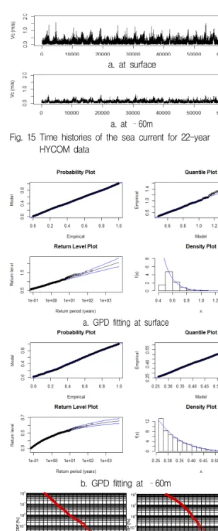
22-year HYCOM time histories of the sea current speed (m/s) at surface and at 60 m below the mean water level are shown in Fig. 15. From the 22-year HYCOM data, the maximum, average and minimum values of the water levels of 0.608 m, 0.183 m and –0.163 m were obtained, respectively. Fig. 16 shows the results of GPD and W3P fittings of the 22-year HYCOM sea current data at surface and 60 m below the mean water level which can be considered unaffected by wind-driven currents. The results of the mean values and extreme value analyses of the 22-year HYCOM sea current data are shown in Table 15. Only the GPD results for extreme values are shown in the table because of the poor W3P fitting. The typhoon-driven current may lead to very high surface sea current speeds.
4. Reduced Design Load Cases
For fully coupled time domain simulations and model tests, the environmental combinations for all DLCs defined in DNVGL-ST-0437:2016, IEC 61400- 3-1:2019 and IEC TS 61400-3-2 have to be deter- mined. At the initial design phase, however, at least the reduced DLCs shown in Table 16 should be considered. In the table, following items are noted:
a) As per DNVGL-RP-C205, were used in the Tp range under normal conditions
Vc(m/s) at surface Vc(m/s) at -60m 22-year
HYCOM data
Max.Min.
Mean
1.580.00 0.22
0.610.00 0.13 Estimated
extremes by GPD
1-year 50-year Threshold
1.161.69 0.48
0.530.62 0.26 Table 15 Mean and extreme value of 22-year HYCOM sea
current data in Donghae gas field a. at surface
a. at –60m
Fig. 15 Time histories of the sea current for 22-year HYCOM data
a. GPD fitting at surface
b. GPD fitting at –60m
Surface Vc [m/s]
1-CDF[%]
0 0.5 1 1.5 2
10-4 10-3 10-2 10-1 100 101 102
W3P Extreme Values:
Shape=0.95500 SScale=0.11910 SLocation=0.43767
Vc [m/s] at -60m
1-CDF[%]
0 0.2 0.4 0.6 0.8
10-4 10-3 10-2 10-1 100 101 102
W3P Extreme Values:
Shape=1.44735 SScale=0.09073 SLocation=0.25511
c. W3P fitting at surface d. W3P fitting at –60m Fig. 16 GPD and W3P fittings of 22-year HYCOM data a: threshold=0.48m/s, n(POT)=4415, D=0.022, p-value=0.217, tie b: threshold=0.26m/s, n(POT)=4138, D=0.037, p-value=0.007, tie c: threshold=0.48m/s, n(POT)=4208, D=0.052, p-value=2.02e-05 d: threshold=0.26m/s, n(POT)=4138, D=0.084, p-value=4.61e-13
![Table 2 50-year extreme conditions of Donghae gas field [5, 6]](https://thumb-ap.123doks.com/thumbv2/123dokinfo/5267173.633265/2.892.418.720.742.982/table-year-extreme-conditions-donghae-gas-field.webp)